CS 4803 7643 Deep Learning Topics Convolutional Neural

CS 4803 / 7643: Deep Learning Topics: – Convolutional Neural Networks – Pooling layers – Fully-connected layers as convolutions – Backprop in conv layers [Derived in notes] – Toeplitz matrices and convolutions = matrix-mult Dhruv Batra Georgia Tech

Administrativia • HW 2 Reminder – Due: 09/23, 11: 59 pm – https: //evalai. cloudcv. org/web/challenges/challengepage/684/leaderboard/1853 • Project Teams – https: //gtvaultmy. sharepoint. com/: x: /g/personal/dbatra 8_gatech_edu/EY 4_ 65 XOz. Wt. Ok. XSSz 2 Wgpo. UBY 8 ux 2 g. Y 9 Ps. Rz. R 6 Kngl. IFEQ? e= 4 tn. KWI – Project Title – 1 -3 sentence project summary TL; DR – Team member names (C) Dhruv Batra 2

Recap from last time (C) Dhruv Batra 3

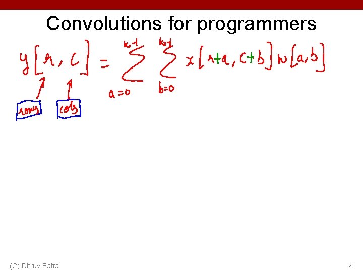
Convolutions for programmers (C) Dhruv Batra 4

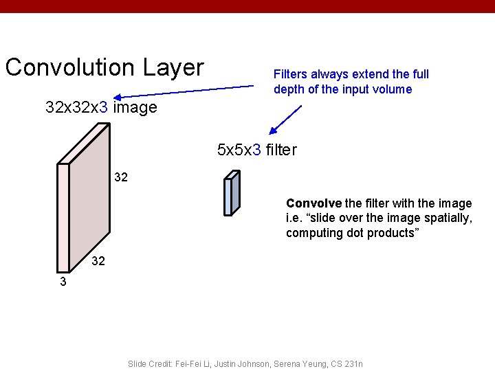
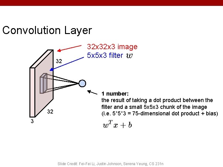
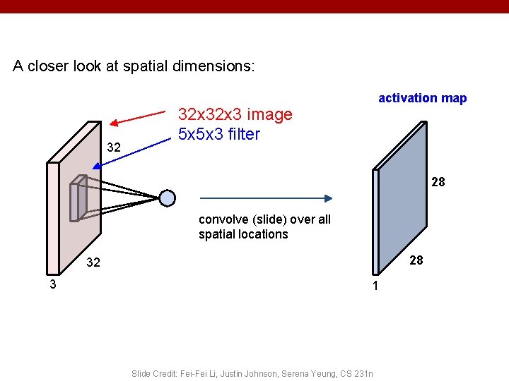
Convolution Layer Filters always extend the full depth of the input volume 32 x 3 image 5 x 5 x 3 filter 32 Convolve the filter with the image i. e. “slide over the image spatially, computing dot products” 32 3 Slide Credit: Fei-Fei Li, Justin Johnson, Serena Yeung, CS 231 n

Convolution Layer 32 32 32 x 3 image 5 x 5 x 3 filter 1 number: the result of taking a dot product between the filter and a small 5 x 5 x 3 chunk of the image (i. e. 5*5*3 = 75 -dimensional dot product + bias) 3 Slide Credit: Fei-Fei Li, Justin Johnson, Serena Yeung, CS 231 n

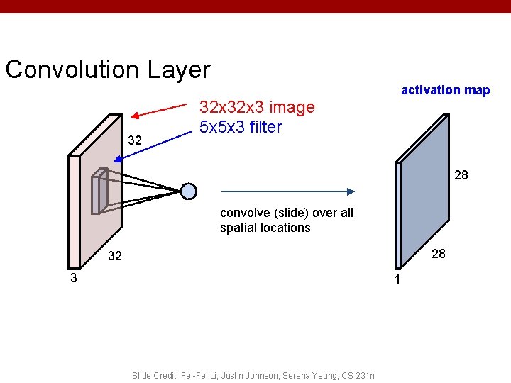
Convolution Layer 32 32 x 3 image 5 x 5 x 3 filter activation map 28 convolve (slide) over all spatial locations 28 32 3 1 Slide Credit: Fei-Fei Li, Justin Johnson, Serena Yeung, CS 231 n

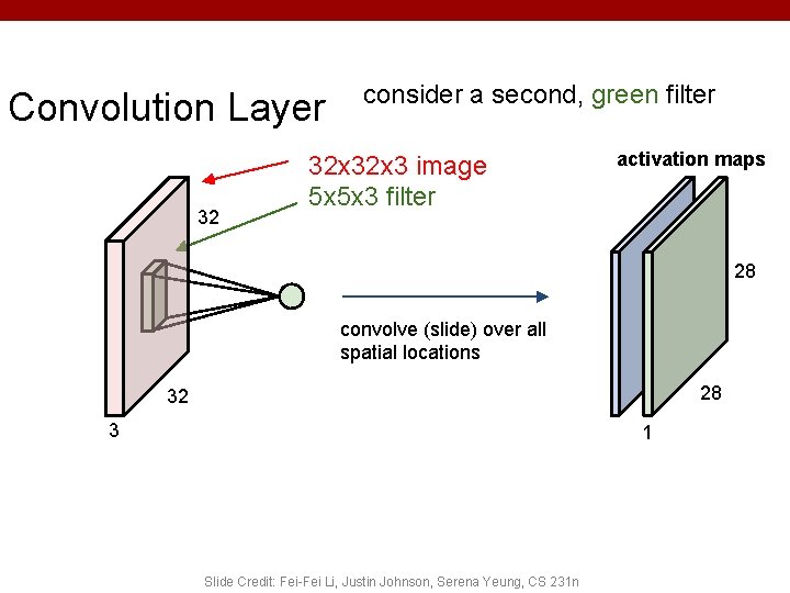
Convolution Layer 32 consider a second, green filter 32 x 3 image 5 x 5 x 3 filter activation maps 28 convolve (slide) over all spatial locations 28 32 3 1 Slide Credit: Fei-Fei Li, Justin Johnson, Serena Yeung, CS 231 n

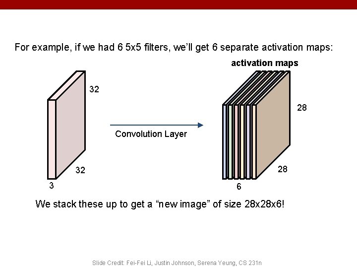
For example, if we had 6 5 x 5 filters, we’ll get 6 separate activation maps: activation maps 32 28 Convolution Layer 28 32 3 6 We stack these up to get a “new image” of size 28 x 6! Slide Credit: Fei-Fei Li, Justin Johnson, Serena Yeung, CS 231 n

Plan for Today • Convolutional Neural Networks – – – (C) Dhruv Batra Stride, padding 1 x 1 convolutions Backprop in conv layers [Derived in notes] Pooling layers Fully-connected layers as convolutions Toeplitz matrices and convolutions = matrix-mult 10

A closer look at spatial dimensions: 32 activation map 32 x 3 image 5 x 5 x 3 filter 28 convolve (slide) over all spatial locations 28 32 3 1 Slide Credit: Fei-Fei Li, Justin Johnson, Serena Yeung, CS 231 n

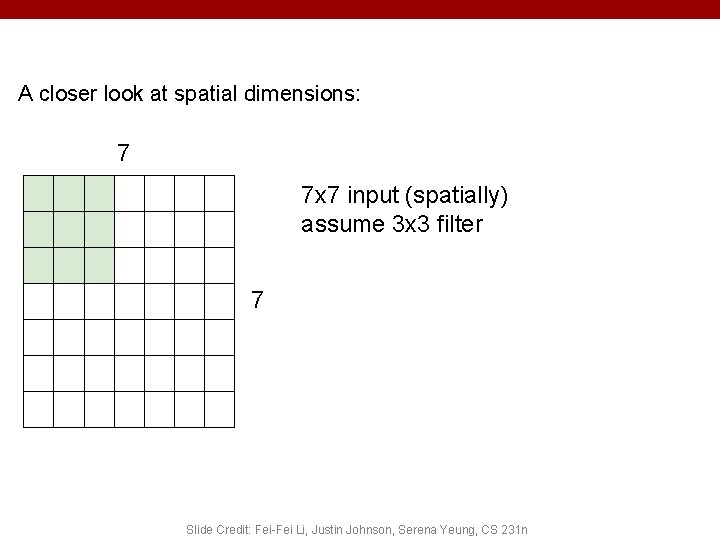
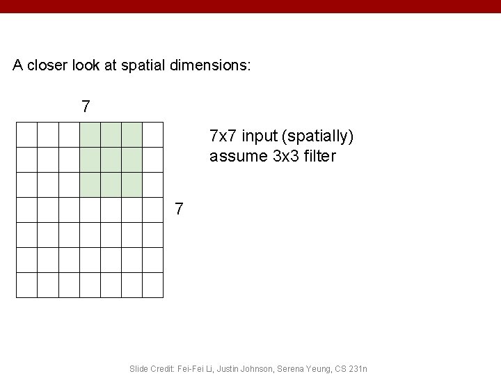
A closer look at spatial dimensions: 7 7 x 7 input (spatially) assume 3 x 3 filter 7 Slide Credit: Fei-Fei Li, Justin Johnson, Serena Yeung, CS 231 n

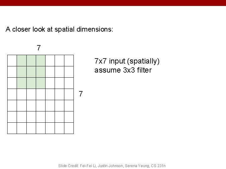
A closer look at spatial dimensions: 7 7 x 7 input (spatially) assume 3 x 3 filter 7 Slide Credit: Fei-Fei Li, Justin Johnson, Serena Yeung, CS 231 n

A closer look at spatial dimensions: 7 7 x 7 input (spatially) assume 3 x 3 filter 7 Slide Credit: Fei-Fei Li, Justin Johnson, Serena Yeung, CS 231 n

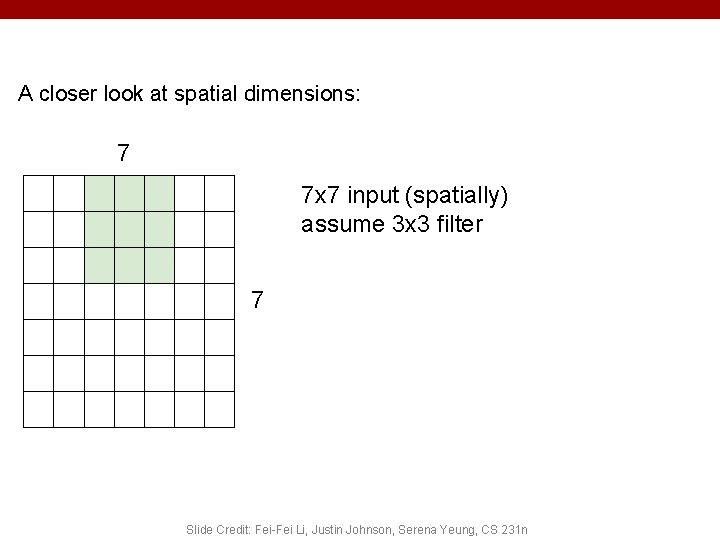
A closer look at spatial dimensions: 7 7 x 7 input (spatially) assume 3 x 3 filter 7 Slide Credit: Fei-Fei Li, Justin Johnson, Serena Yeung, CS 231 n

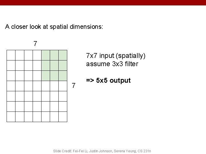
A closer look at spatial dimensions: 7 7 x 7 input (spatially) assume 3 x 3 filter 7 => 5 x 5 output Slide Credit: Fei-Fei Li, Justin Johnson, Serena Yeung, CS 231 n

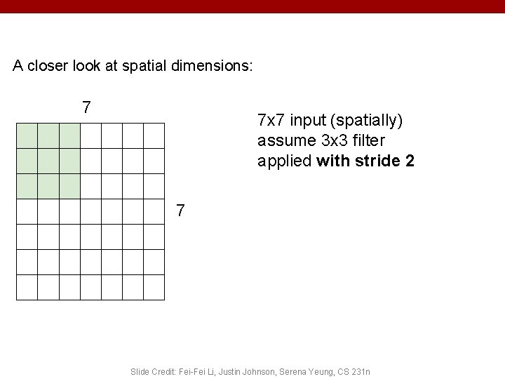
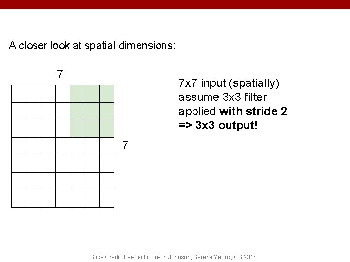
A closer look at spatial dimensions: 7 7 x 7 input (spatially) assume 3 x 3 filter applied with stride 2 7 Slide Credit: Fei-Fei Li, Justin Johnson, Serena Yeung, CS 231 n

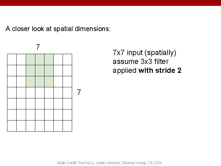
A closer look at spatial dimensions: 7 7 x 7 input (spatially) assume 3 x 3 filter applied with stride 2 7 Slide Credit: Fei-Fei Li, Justin Johnson, Serena Yeung, CS 231 n

A closer look at spatial dimensions: 7 7 x 7 input (spatially) assume 3 x 3 filter applied with stride 2 => 3 x 3 output! 7 Slide Credit: Fei-Fei Li, Justin Johnson, Serena Yeung, CS 231 n

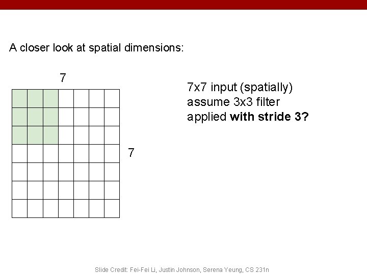
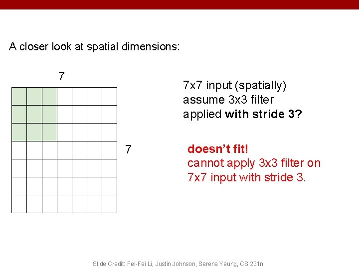
A closer look at spatial dimensions: 7 7 x 7 input (spatially) assume 3 x 3 filter applied with stride 3? 7 Slide Credit: Fei-Fei Li, Justin Johnson, Serena Yeung, CS 231 n

A closer look at spatial dimensions: 7 7 x 7 input (spatially) assume 3 x 3 filter applied with stride 3? 7 doesn’t fit! cannot apply 3 x 3 filter on 7 x 7 input with stride 3. Slide Credit: Fei-Fei Li, Justin Johnson, Serena Yeung, CS 231 n

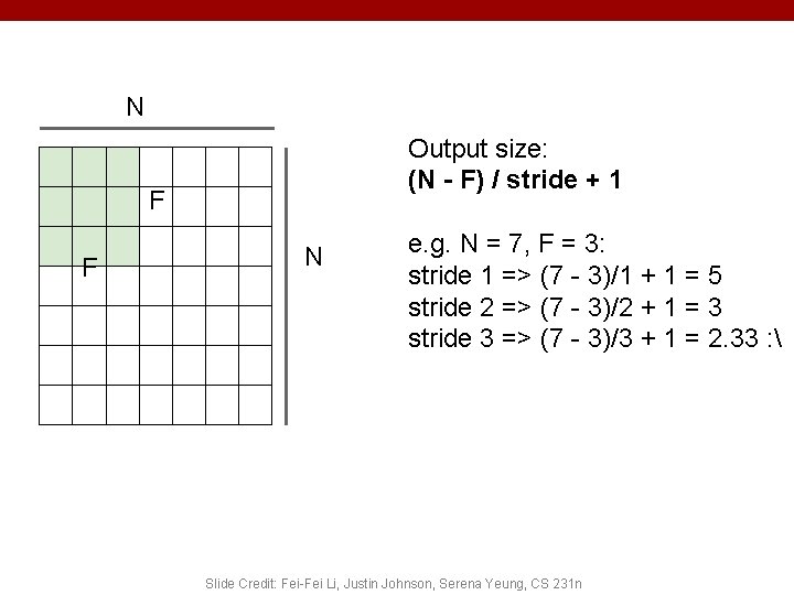
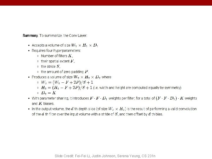
N Output size: (N - F) / stride + 1 F F N e. g. N = 7, F = 3: stride 1 => (7 - 3)/1 + 1 = 5 stride 2 => (7 - 3)/2 + 1 = 3 stride 3 => (7 - 3)/3 + 1 = 2. 33 : Slide Credit: Fei-Fei Li, Justin Johnson, Serena Yeung, CS 231 n

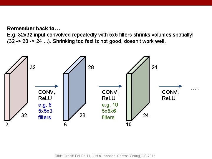
Remember back to… E. g. 32 x 32 input convolved repeatedly with 5 x 5 filters shrinks volumes spatially! (32 -> 28 -> 24. . . ). Shrinking too fast is not good, doesn’t work well. 32 32 3 28 CONV, Re. LU e. g. 6 5 x 5 x 3 filters 28 6 24 CONV, Re. LU e. g. 10 5 x 5 x 6 filters CONV, Re. LU 24 10 Slide Credit: Fei-Fei Li, Justin Johnson, Serena Yeung, CS 231 n ….

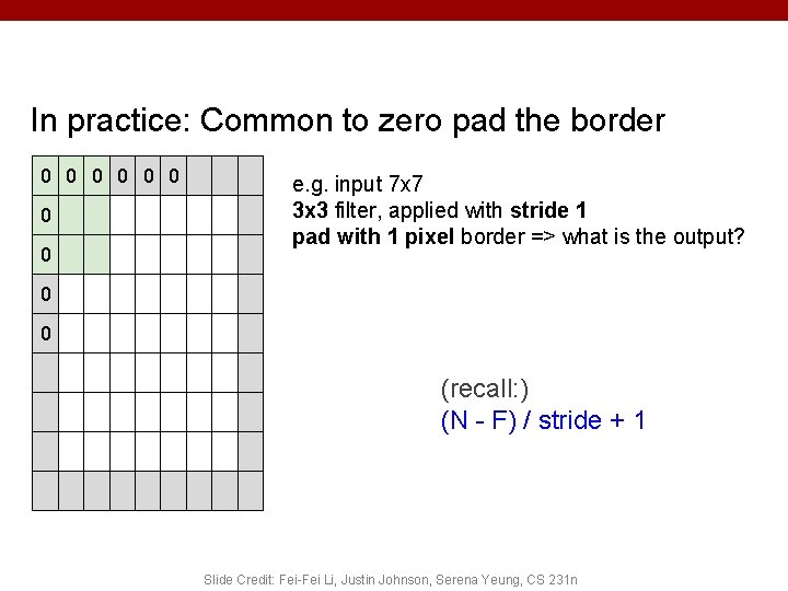
In practice: Common to zero pad the border 0 0 0 0 e. g. input 7 x 7 3 x 3 filter, applied with stride 1 pad with 1 pixel border => what is the output? 0 0 (recall: ) (N - F) / stride + 1 Slide Credit: Fei-Fei Li, Justin Johnson, Serena Yeung, CS 231 n

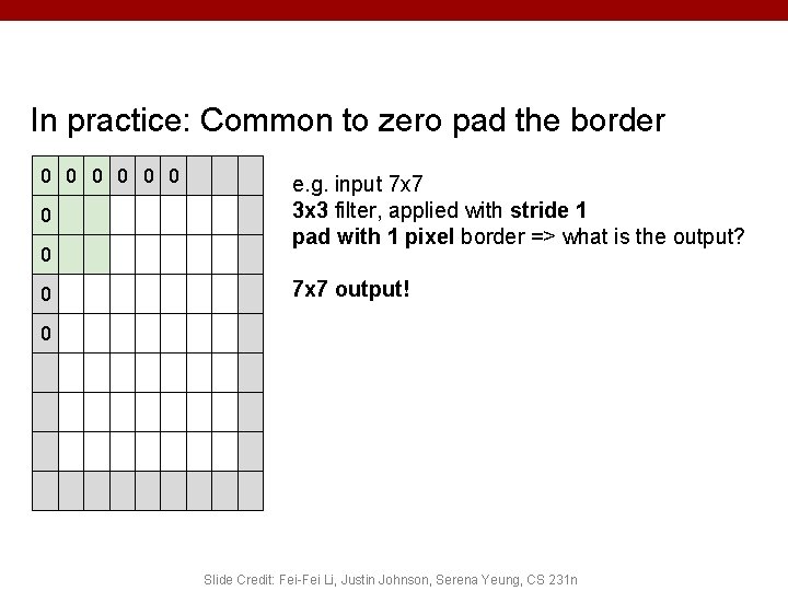
In practice: Common to zero pad the border 0 0 0 0 0 e. g. input 7 x 7 3 x 3 filter, applied with stride 1 pad with 1 pixel border => what is the output? 7 x 7 output! 0 Slide Credit: Fei-Fei Li, Justin Johnson, Serena Yeung, CS 231 n

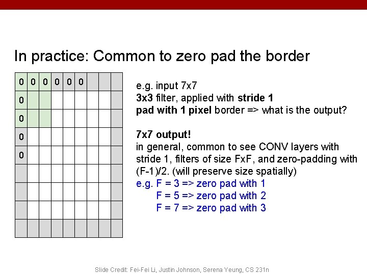
In practice: Common to zero pad the border 0 0 0 0 0 e. g. input 7 x 7 3 x 3 filter, applied with stride 1 pad with 1 pixel border => what is the output? 7 x 7 output! in general, common to see CONV layers with stride 1, filters of size Fx. F, and zero-padding with (F-1)/2. (will preserve size spatially) e. g. F = 3 => zero pad with 1 F = 5 => zero pad with 2 F = 7 => zero pad with 3 Slide Credit: Fei-Fei Li, Justin Johnson, Serena Yeung, CS 231 n

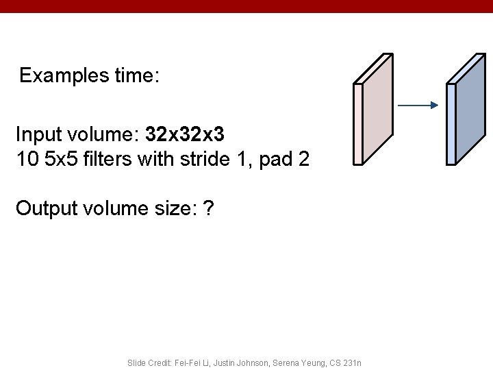
Examples time: Input volume: 32 x 3 10 5 x 5 filters with stride 1, pad 2 Output volume size: ? Slide Credit: Fei-Fei Li, Justin Johnson, Serena Yeung, CS 231 n

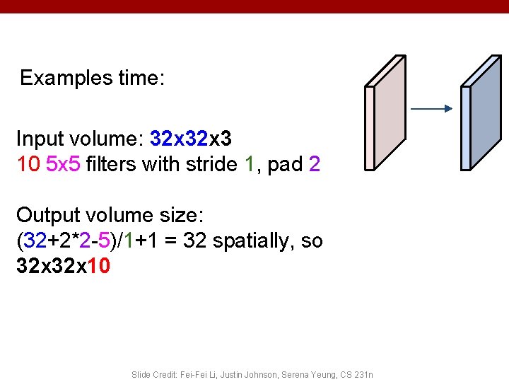
Examples time: Input volume: 32 x 3 10 5 x 5 filters with stride 1, pad 2 Output volume size: (32+2*2 -5)/1+1 = 32 spatially, so 32 x 10 Slide Credit: Fei-Fei Li, Justin Johnson, Serena Yeung, CS 231 n

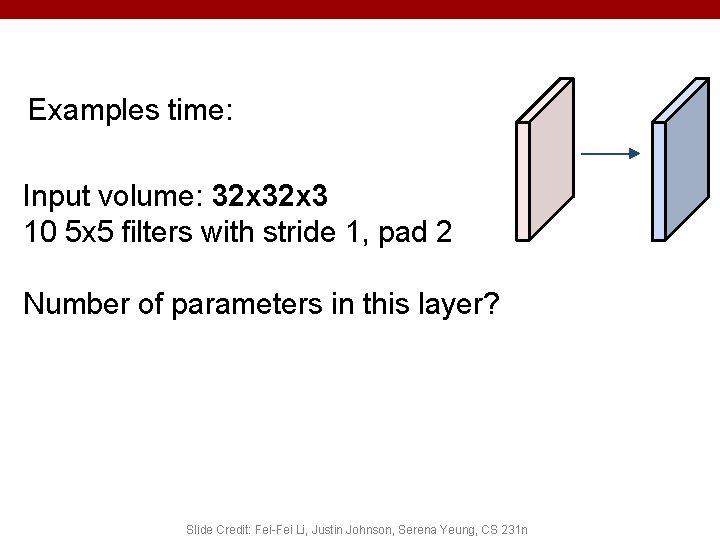
Examples time: Input volume: 32 x 3 10 5 x 5 filters with stride 1, pad 2 Number of parameters in this layer? Slide Credit: Fei-Fei Li, Justin Johnson, Serena Yeung, CS 231 n

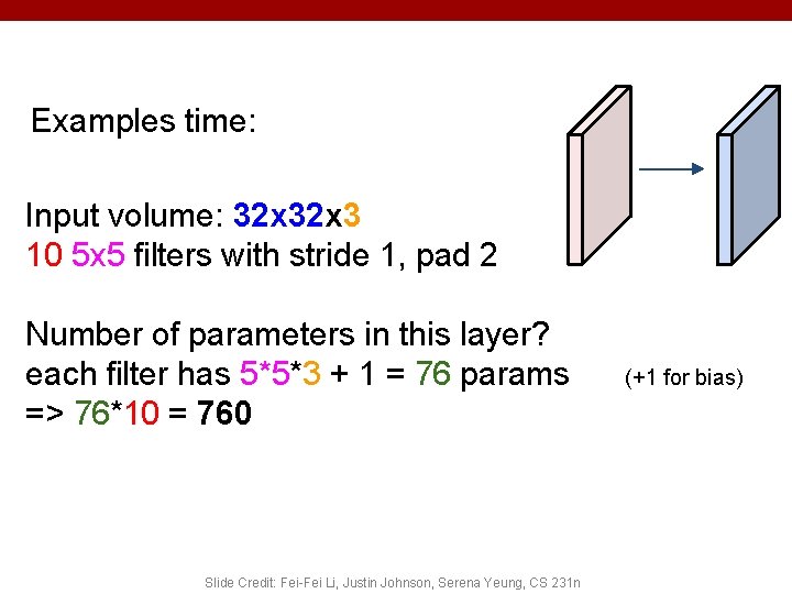
Examples time: Input volume: 32 x 3 10 5 x 5 filters with stride 1, pad 2 Number of parameters in this layer? each filter has 5*5*3 + 1 = 76 params => 76*10 = 760 Slide Credit: Fei-Fei Li, Justin Johnson, Serena Yeung, CS 231 n (+1 for bias)

Slide Credit: Fei-Fei Li, Justin Johnson, Serena Yeung, CS 231 n

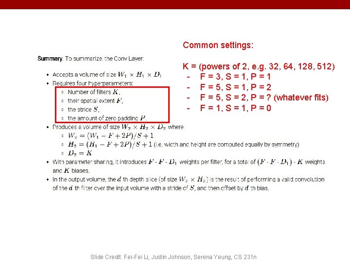
Common settings: K = (powers of 2, e. g. 32, 64, 128, 512) - F = 3, S = 1, P = 1 - F = 5, S = 1, P = 2 - F = 5, S = 2, P = ? (whatever fits) - F = 1, S = 1, P = 0 Slide Credit: Fei-Fei Li, Justin Johnson, Serena Yeung, CS 231 n

Plan for Today • Convolutional Neural Networks – – – (C) Dhruv Batra Stride, padding 1 x 1 convolutions Backprop in conv layers [Derived in notes] Pooling layers Fully-connected layers as convolutions Toeplitz matrices and convolutions = matrix-mult 34

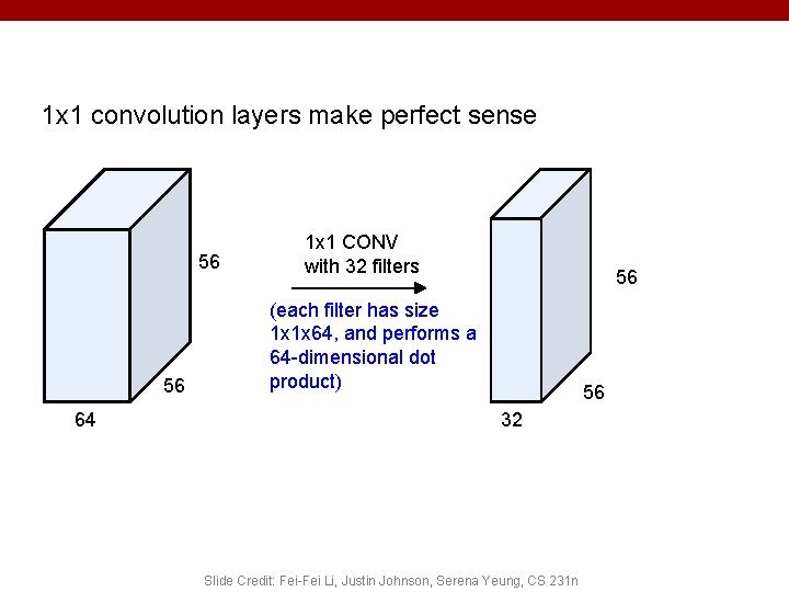
Can we have 1 x 1 filters? (C) Dhruv Batra 35

1 x 1 convolution layers make perfect sense 56 56 64 1 x 1 CONV with 32 filters 56 (each filter has size 1 x 1 x 64, and performs a 64 -dimensional dot product) 56 32 Slide Credit: Fei-Fei Li, Justin Johnson, Serena Yeung, CS 231 n

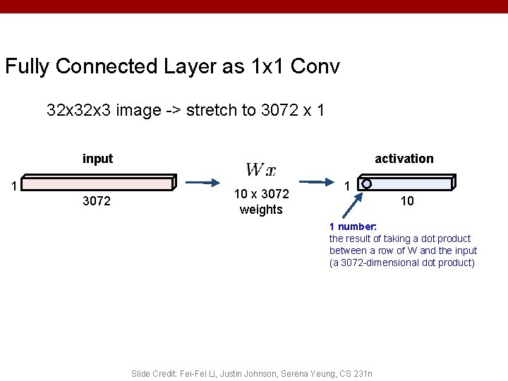
Fully Connected Layer as 1 x 1 Conv 32 x 3 image -> stretch to 3072 x 1 input 1 3072 activation 10 x 3072 weights 1 10 1 number: the result of taking a dot product between a row of W and the input (a 3072 -dimensional dot product) Slide Credit: Fei-Fei Li, Justin Johnson, Serena Yeung, CS 231 n

Plan for Today • Convolutional Neural Networks – – – (C) Dhruv Batra Stride, padding 1 x 1 convolutions Backprop in conv layers [Derived in notes] Pooling layers Fully-connected layers as convolutions Toeplitz matrices and convolutions = matrix-mult 38

Computational Graph Any DAG of differentiable modules is allowed! (C) Dhruv Batra Slide Credit: Marc'Aurelio Ranzato 39

Key Computation: Forward-Prop (C) Dhruv Batra Slide Credit: Marc'Aurelio Ranzato, Yann Le. Cun 40

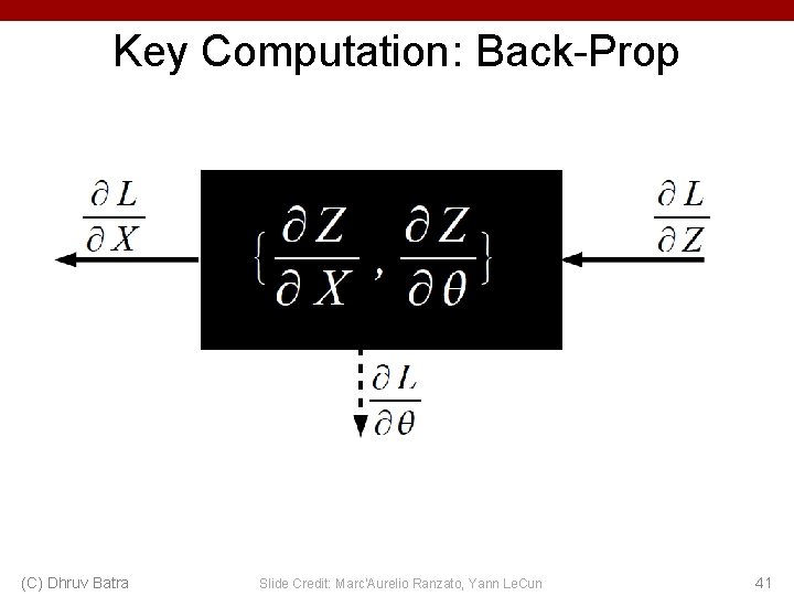
Key Computation: Back-Prop (C) Dhruv Batra Slide Credit: Marc'Aurelio Ranzato, Yann Le. Cun 41

Backprop in Convolutional Layers • Notes – https: //www. cc. gatech. edu/classes/AY 2021/cs 7643_fall/slide s/L 11_cnns_backprop_notes. pdf (C) Dhruv Batra 42

Backprop in Convolutional Layers (C) Dhruv Batra 43

Backprop in Convolutional Layers (C) Dhruv Batra 44

Backprop in Convolutional Layers (C) Dhruv Batra 45

Plan for Today • Convolutional Neural Networks – – – (C) Dhruv Batra Stride, padding 1 x 1 convolutions Backprop in conv layers [Derived in notes] Pooling layers Fully-connected layers as convolutions Toeplitz matrices and convolutions = matrix-mult 46

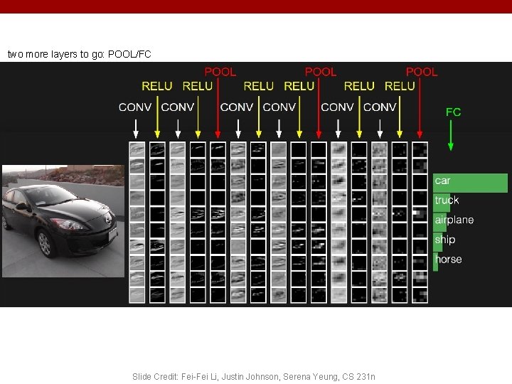
two more layers to go: POOL/FC Slide Credit: Fei-Fei Li, Justin Johnson, Serena Yeung, CS 231 n

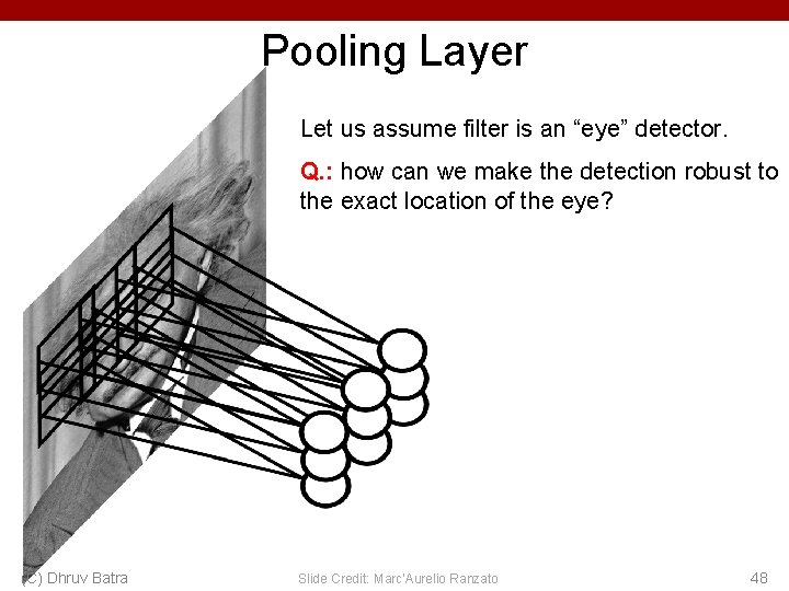
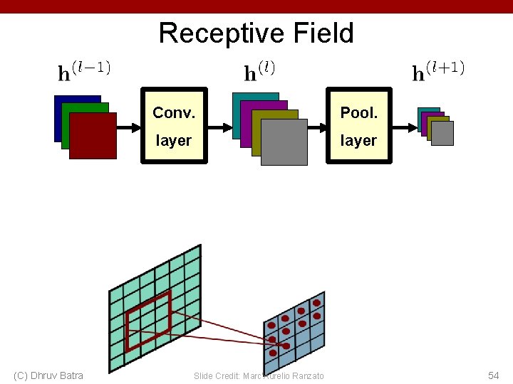
Pooling Layer Let us assume filter is an “eye” detector. Q. : how can we make the detection robust to the exact location of the eye? (C) Dhruv Batra Slide Credit: Marc'Aurelio Ranzato 48

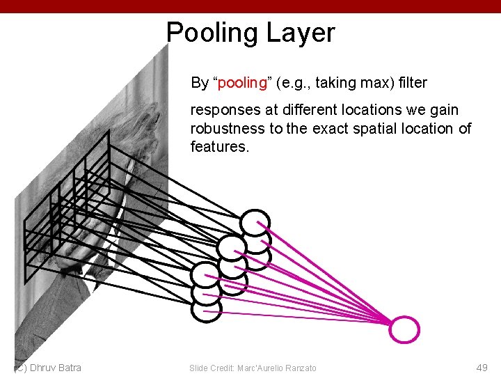
Pooling Layer By “pooling” (e. g. , taking max) filter responses at different locations we gain robustness to the exact spatial location of features. (C) Dhruv Batra Slide Credit: Marc'Aurelio Ranzato 49

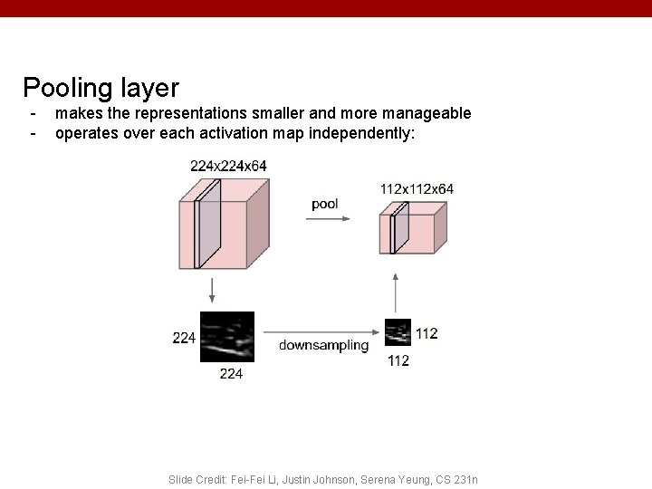
Pooling layer - makes the representations smaller and more manageable operates over each activation map independently: Slide Credit: Fei-Fei Li, Justin Johnson, Serena Yeung, CS 231 n

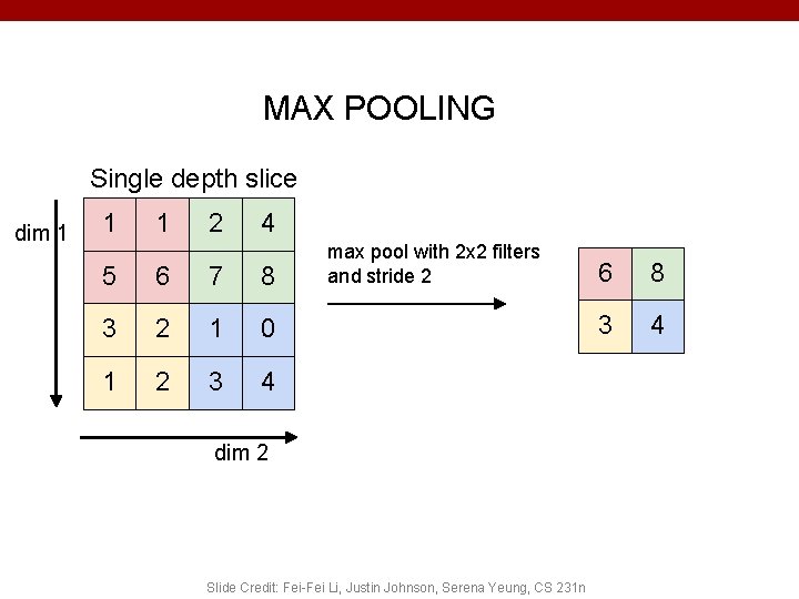
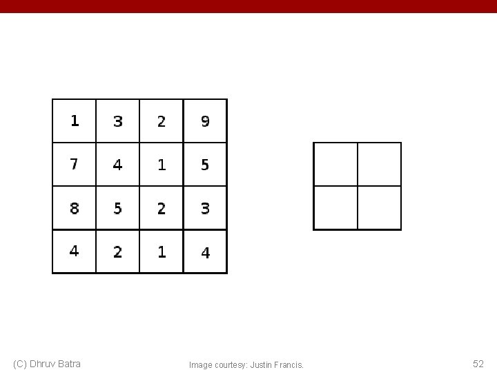
MAX POOLING Single depth slice dim 1 1 1 2 4 5 6 7 8 3 2 1 0 1 2 3 4 max pool with 2 x 2 filters and stride 2 dim 2 Slide Credit: Fei-Fei Li, Justin Johnson, Serena Yeung, CS 231 n 6 8 3 4

(C) Dhruv Batra Image courtesy: Justin Francis. 52

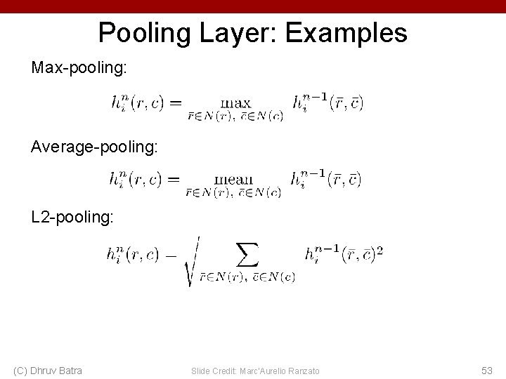
Pooling Layer: Examples Max-pooling: Average-pooling: L 2 -pooling: (C) Dhruv Batra Slide Credit: Marc'Aurelio Ranzato 53

Receptive Field (C) Dhruv Batra Conv. Pool. layer Slide Credit: Marc'Aurelio Ranzato 54

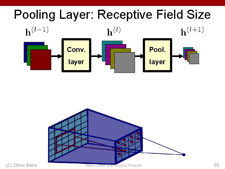
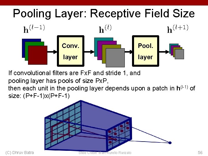
Pooling Layer: Receptive Field Size (C) Dhruv Batra Conv. Pool. layer Slide Credit: Marc'Aurelio Ranzato 55

Pooling Layer: Receptive Field Size Conv. Pool. layer If convolutional filters are Fx. F and stride 1, and pooling layer has pools of size Px. P, then each unit in the pooling layer depends upon a patch in h(l-1) of size: (P+F-1)x(P+F-1) (C) Dhruv Batra Slide Credit: Marc'Aurelio Ranzato 56

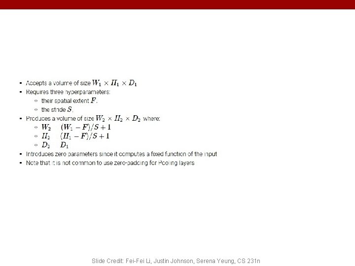
Slide Credit: Fei-Fei Li, Justin Johnson, Serena Yeung, CS 231 n

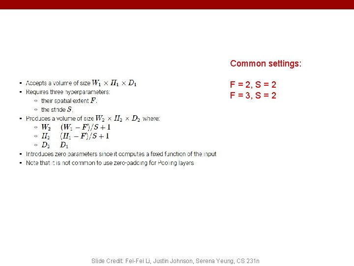
Common settings: F = 2, S = 2 F = 3, S = 2 Slide Credit: Fei-Fei Li, Justin Johnson, Serena Yeung, CS 231 n

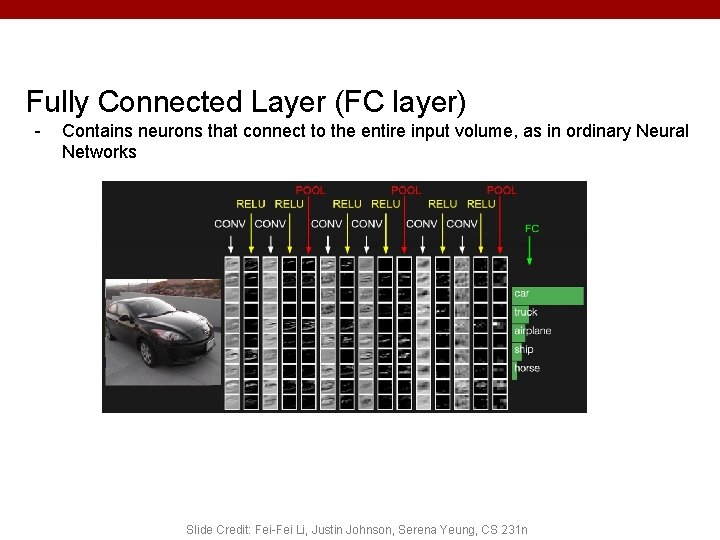
Fully Connected Layer (FC layer) - Contains neurons that connect to the entire input volume, as in ordinary Neural Networks Slide Credit: Fei-Fei Li, Justin Johnson, Serena Yeung, CS 231 n

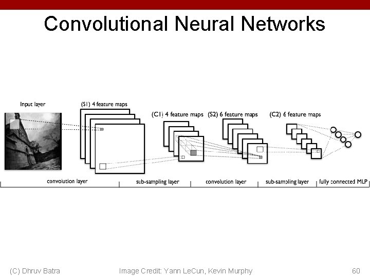
Convolutional Neural Networks (C) Dhruv Batra Image Credit: Yann Le. Cun, Kevin Murphy 60

Classical View (C) Dhruv Batra Figure Credit: [Long, Shelhamer, Darrell CVPR 15] 61

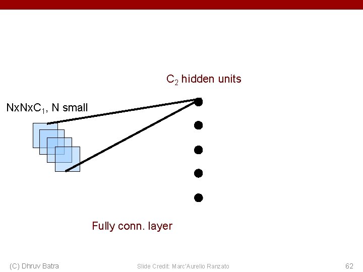
C 2 hidden units Nx. C 1, N small Fully conn. layer (C) Dhruv Batra Slide Credit: Marc'Aurelio Ranzato 62

Classical View (C) Dhruv Batra Figure Credit: [Long, Shelhamer, Darrell CVPR 15] 63

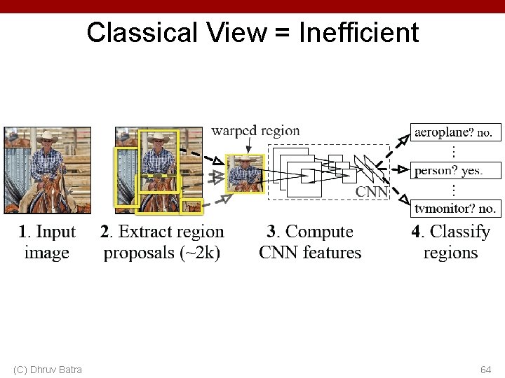
Classical View = Inefficient (C) Dhruv Batra 64

Classical View (C) Dhruv Batra Figure Credit: [Long, Shelhamer, Darrell CVPR 15] 65

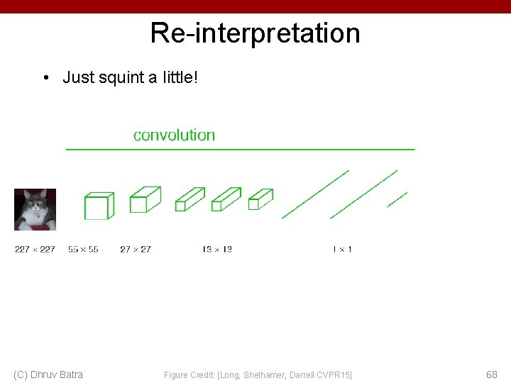
Re-interpretation • Just squint a little! (C) Dhruv Batra Figure Credit: [Long, Shelhamer, Darrell CVPR 15] 66

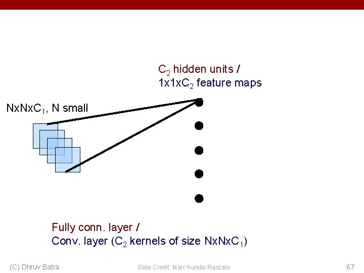
C 2 hidden units / 1 x 1 x. C 2 feature maps Nx. C 1, N small Fully conn. layer / Conv. layer (C 2 kernels of size Nx. C 1) (C) Dhruv Batra Slide Credit: Marc'Aurelio Ranzato 67

Re-interpretation • Just squint a little! (C) Dhruv Batra Figure Credit: [Long, Shelhamer, Darrell CVPR 15] 68

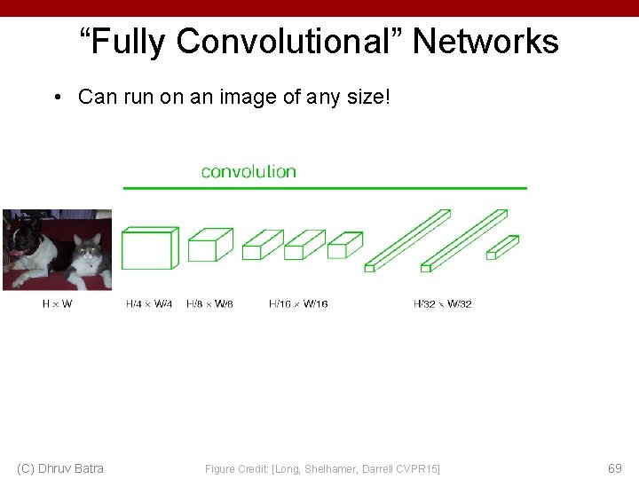
“Fully Convolutional” Networks • Can run on an image of any size! (C) Dhruv Batra Figure Credit: [Long, Shelhamer, Darrell CVPR 15] 69

Benefit of this thinking • Mathematically elegant • Efficiency – Can run network on arbitrary image – Without multiple crops (C) Dhruv Batra 71

Plan for Today • Convolutional Neural Networks – – – (C) Dhruv Batra Stride, padding 1 x 1 convolutions Backprop in conv layers [Derived in notes] Pooling layers Fully-connected layers as convolutions Toeplitz matrices and convolutions = matrix-mult 72

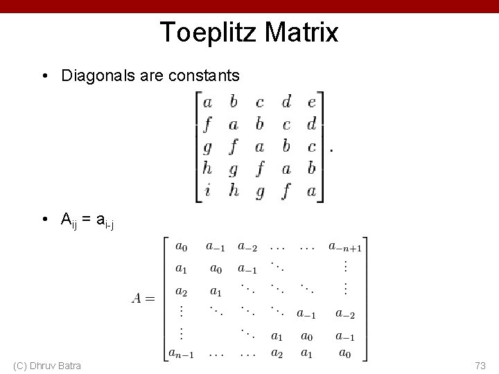
Toeplitz Matrix • Diagonals are constants • Aij = ai-j (C) Dhruv Batra 73

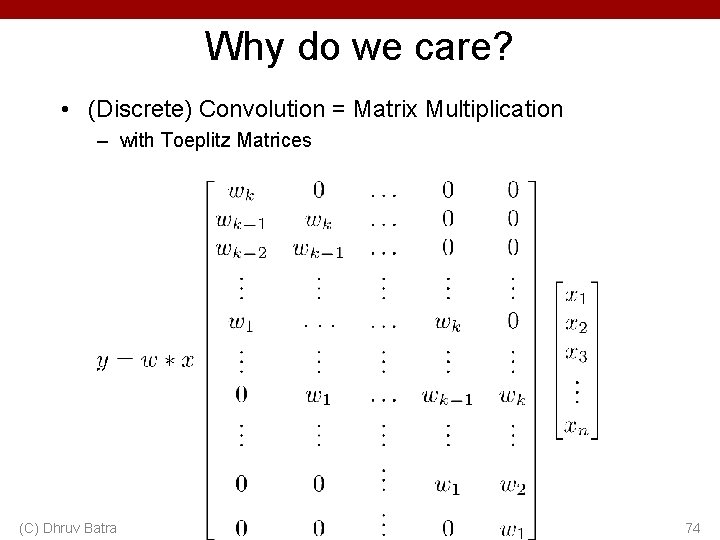
Why do we care? • (Discrete) Convolution = Matrix Multiplication – with Toeplitz Matrices . . . (C) Dhruv Batra 74

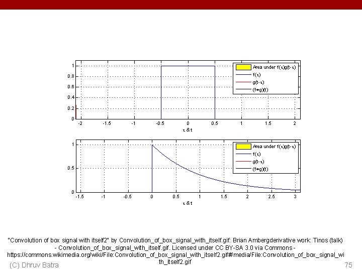
"Convolution of box signal with itself 2" by Convolution_of_box_signal_with_itself. gif: Brian Ambergderivative work: Tinos (talk) - Convolution_of_box_signal_with_itself. gif. Licensed under CC BY-SA 3. 0 via Commons https: //commons. wikimedia. org/wiki/File: Convolution_of_box_signal_with_itself 2. gif#/media/File: Convolution_of_box_signal_wi th_itself 2. gif (C) Dhruv Batra 75

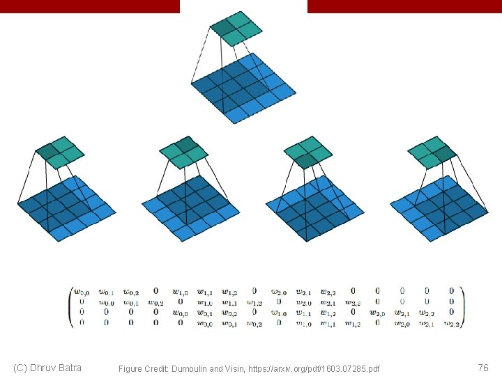
(C) Dhruv Batra Figure Credit: Dumoulin and Visin, https: //arxiv. org/pdf/1603. 07285. pdf 76