Inventory Management and Risk Pooling Tokyo University of

Inventory Management and Risk Pooling Tokyo University of Marine Science and Technology Mikio Kubo

Why the inventory management is so important? • GM reduced their inventory and transportation costs by 26% using a decision support tool that optimizes their fright shipment schedule. • In 1994, IBM struggled with shortages in the Think. Pad line due to ineffective inventory management • The average inventory levels of Japanese super markets are 2 weeks in food, 4 weeks in non-food products.

Two basic laws in inventory management • The first law The demand forecast is always wrong. • The second law The aggregation of inventories reduces the total amount of inventories Other reasons for holding inventories are: • Economy of scale in production and/or transportation (lot-sizing inventories) • Uncertainty of the lead time • To catch up with the seasonal demand (seasonal inventories)

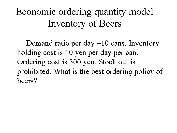
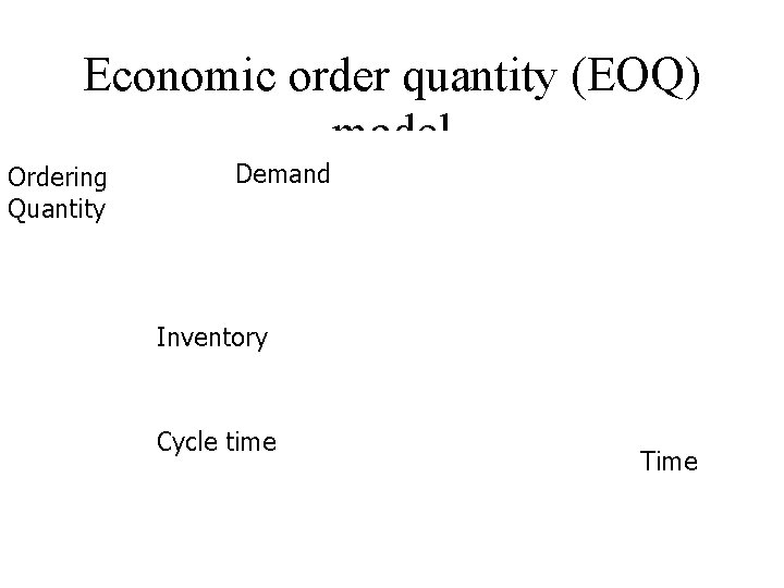
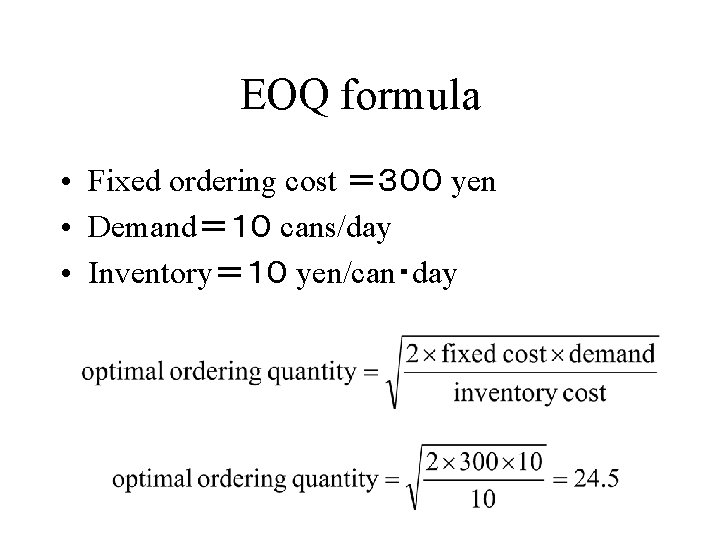
Economic ordering quantity model Inventory of Beers 　　　Demand ratio per day =10 cans. Inventory holding cost is 10 yen per day per can. Ordering cost is 300 yen. Stock out is prohibited. What is the best ordering policy of beers?

Economic order quantity (EOQ) model Ordering Quantity Demand Inventory Cycle time Time

EOQ formula • Fixed ordering cost ＝３００ yen • Demand＝１０ cans/day • Inventory＝１０ yen/can・day

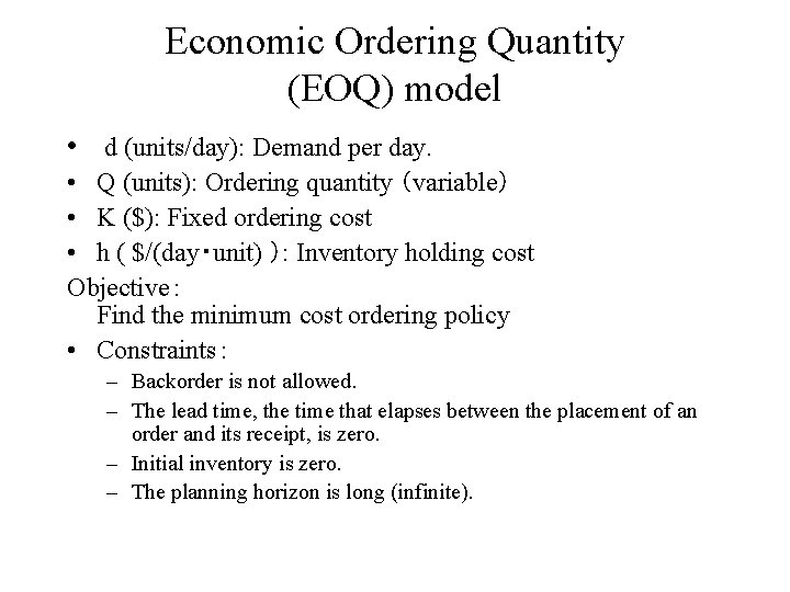
Economic Ordering Quantity (EOQ) model • d (units/day): Demand per day. • Q (units): Ordering quantity （variable） • K ($): Fixed ordering cost • h ( $/(day・unit) ）: Inventory holding cost Objective： Find the minimum cost ordering policy • Constraints： – Backorder is not allowed． – The lead time, the time that elapses between the placement of an order and its receipt, is zero. – Initial inventory is zero. – The planning horizon is long (infinite).

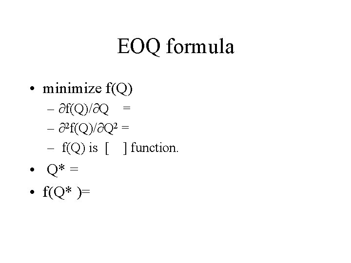
Inventory level d：demand speed Q h×Area Cycle time (T days) = [ ] Time Total cost over T days = Ordering cost +Inventory Cost = f(Q)= Cost per day =

EOQ formula • minimize f(Q) – ∂f(Q)/∂Q = – ∂2 f(Q)/∂Q 2 = – f(Q) is [ ] function. • Q* = • f(Q* )=

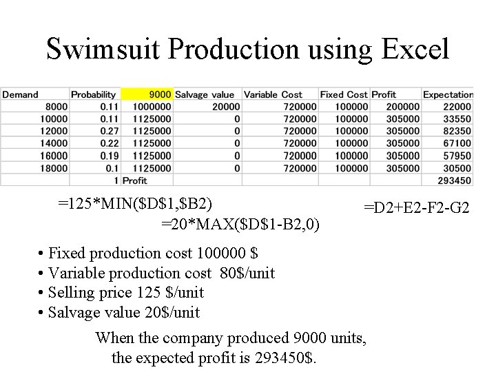
Swimsuit Production using Excel =125*MIN($D$1, $B 2) =20*MAX($D$1 -B 2, 0) =D 2+E 2 -F 2 -G 2 • Fixed production cost 100000 $ • Variable production cost 80$/unit • Selling price 125 $/unit • Salvage value 20$/unit When the company produced 9000 units, the expected profit is 293450$.

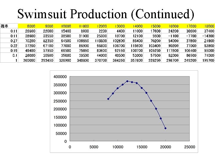
Swimsuit Production (Continued)

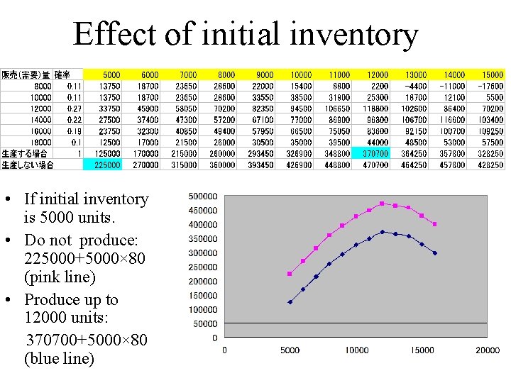
Effect of initial inventory • If initial inventory is 5000 units. • Do not produce: 225000+5000× 80 (pink line) • Produce up to 12000 units: 370700+5000× 80 (blue line)

Truncated Normal distribution with mean 100 and standard deviation 100 Probability density function Demand

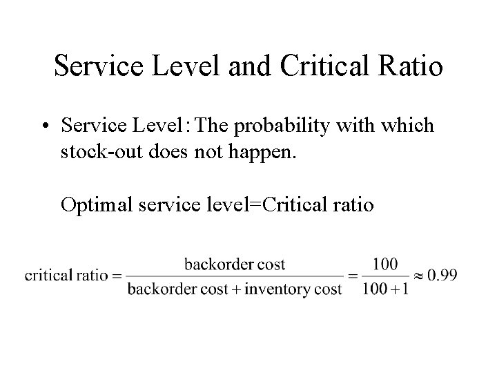
Service Level and Critical Ratio • Service Level：The probability with which stock-out does not happen. Optimal service level=Critical ratio

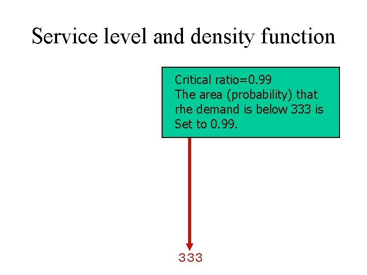
Service level and density function Critical ratio=0. 99 The area (probability) that rhe demand is below 333 is Set to 0. 99. ３３３

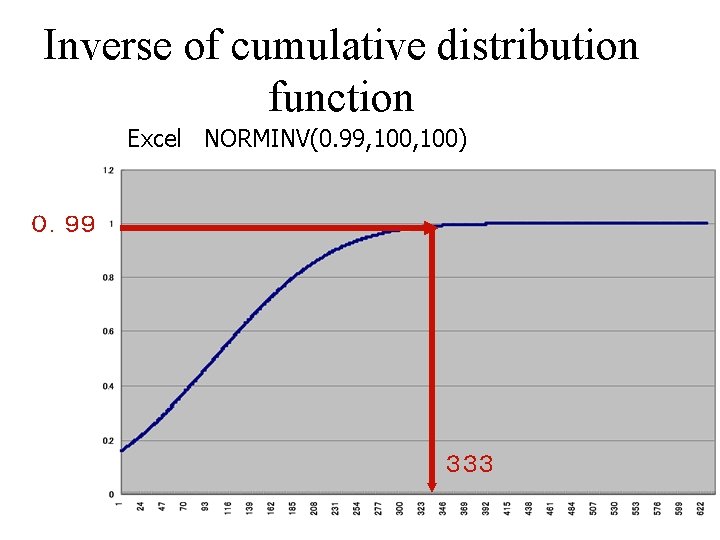
Inverse of cumulative distribution function Excel NORMINV(0. 99, 100) ０．９９ ３３３

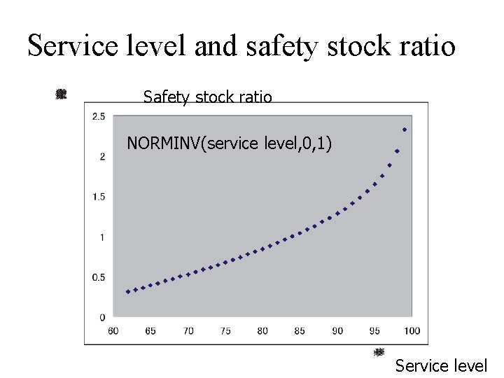
Service level and safety stock ratio Safety stock ratio NORMINV(service level, 0, 1) Service level

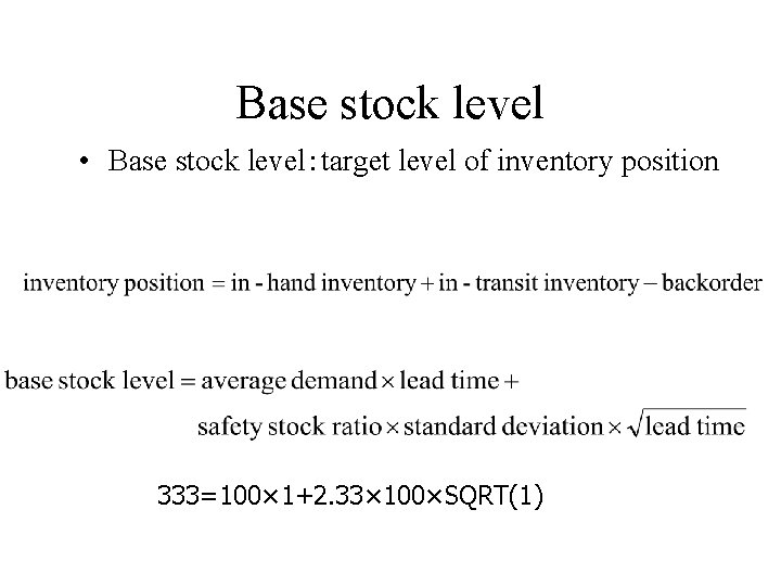
Base stock level • Base stock level：target level of inventory position 333=100× 1+2. 33× 100×SQRT(1)

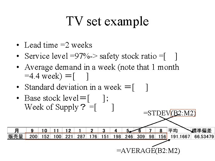
TV set example • Lead time =2 weeks • Service level =97%-> safety stock ratio =[ ] • Average demand in a week (note that 1 month =4. 4 week) ＝[ ] • Standard deviation in a week ＝[ ] • Base stock level＝[ ]； Week of Supply？ =[ ] =STDEV(B 2: M 2) =AVERAGE(B 2: M 2)

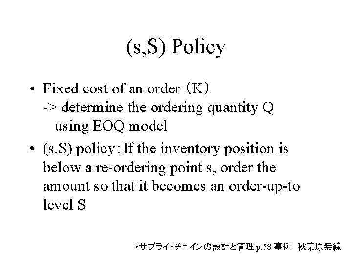
(s, S) Policy • Fixed cost of an order （K） -> determine the ordering quantity Q using EOQ model • (s, S) policy：If the inventory position is below a re-ordering point s, order the amount so that it becomes an order-up-to level S • サプライ・チェインの設計と管理 p. 58 事例　秋葉原無線

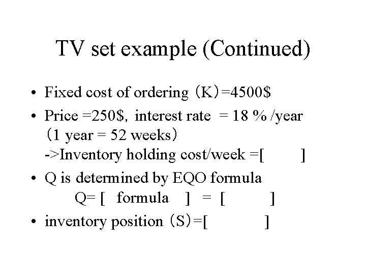
TV set example (Continued) • Fixed cost of ordering （K）=4500$ • Price =250$，interest rate = 18 % /year （1 year = 52 weeks） ->Inventory holding cost/week =[ ] • Q is determined by EQO formula 　　 Q= [ formula ] = [ ] • inventory position （S）=[ ]

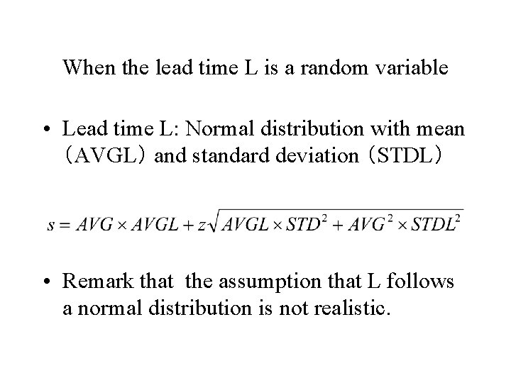
When the lead time L is a random variable • Lead time L: Normal distribution with mean （AVGL） and standard deviation （STDL） • Remark that the assumption that L follows a normal distribution is not realistic.

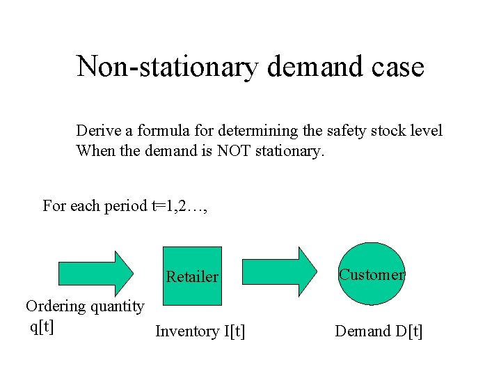
Non-stationary demand case Derive a formula for determining the safety stock level When the demand is NOT stationary. For each period t=1, 2…, Retailer Ordering quantity q[t] Inventory I[t] Customer Demand D[t]

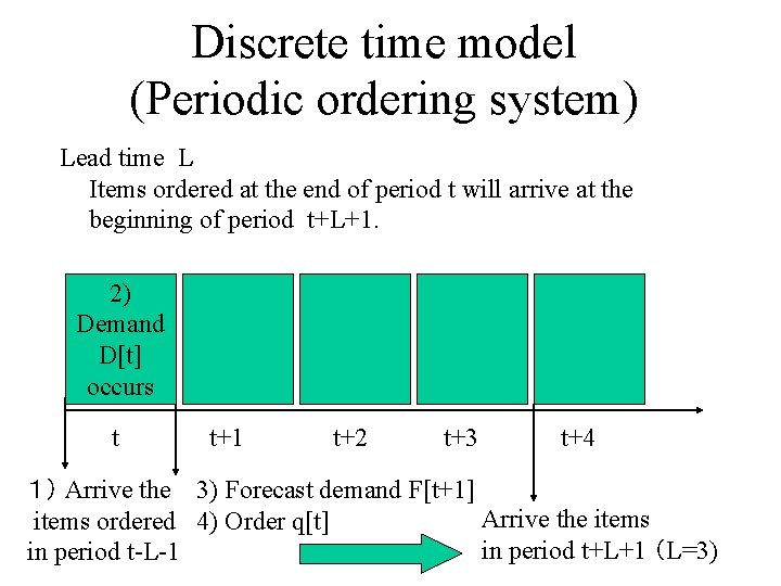
Discrete time model (Periodic ordering system) Lead time L Items ordered at the end of period t will arrive at the beginning of period t+L+1. 2) Demand D[t] occurs t t+1 t+2 t+3 t+4 １） Arrive the 3) Forecast demand F[t+1] Arrive the items ordered 4) Order q[t] in period t+L+1 （L=3) in period t-L-1

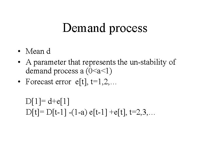
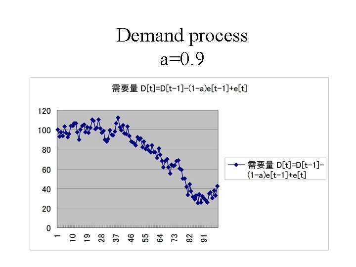
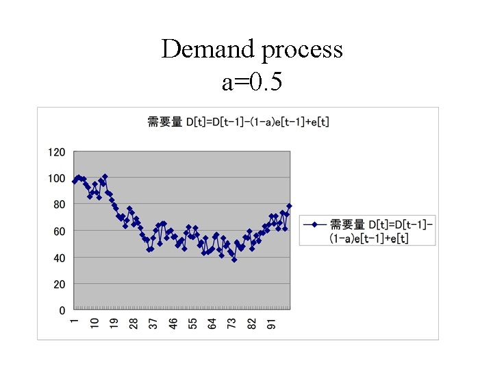
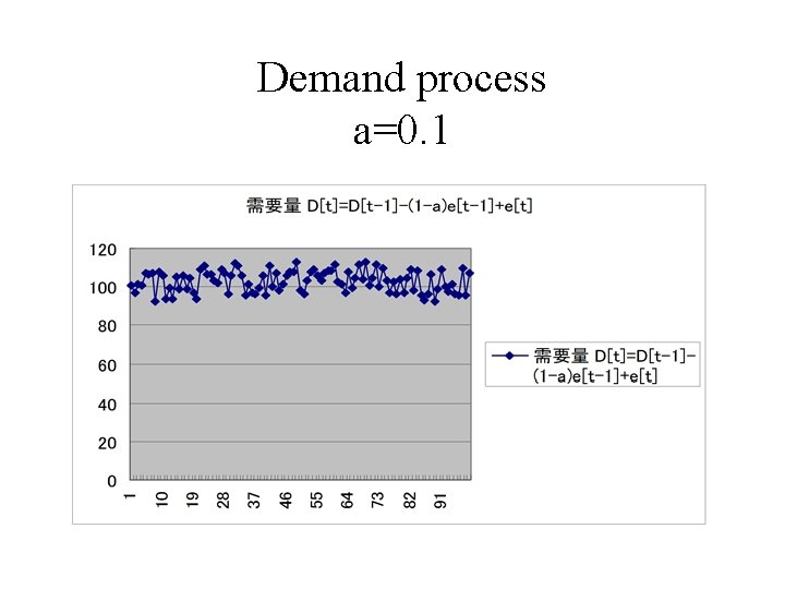
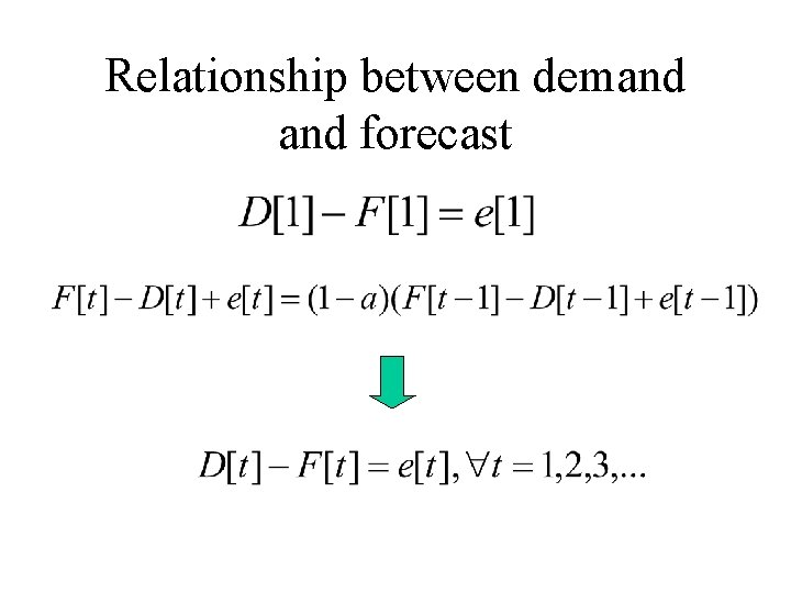
Demand process • Mean d • A parameter that represents the un-stability of demand process a (0<a<1) • Forecast error e[t], t=1, 2, … D[1]= d+e[1] D[t]= D[t-1] -(1 -a) e[t-1] +e[t], t=2, 3, …

Excel d=100, a=0. 9, e[t]=[-10, 10] (uniform r. v. ) １ ２ ３ ４ ５ ６ ７ A =100+B 2 B =RAND()*(-20)+10 =A 2 -（１－C 2）*B 2+B 3 C =C 3

Demand process a=0. 9

Demand process a=0. 5

Demand process a=0. 1

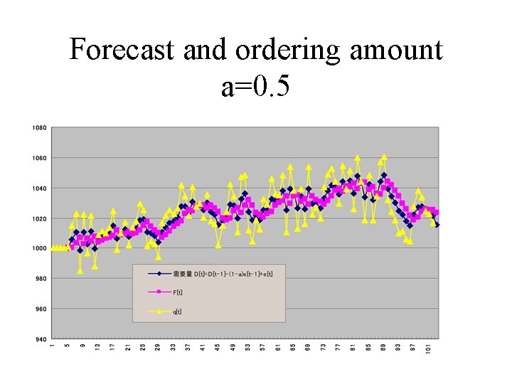
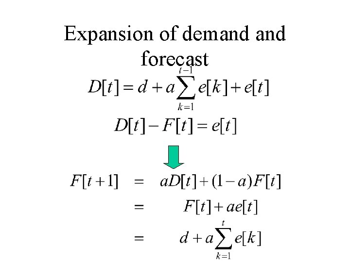
Ordering quantity q[t] • Forecast future demands (exponential smoothing method） F[1]=d F[t]=a D[t-1] + (1 -a) F[t-1], t=2, 3, … • Ordering quantity: At the end of period t, order the amount q[t]=D[t]+(L+1) (F[t+1]-F[t]) , t=1, 2, … where q[t]=d, t<=0.

Forecast and ordering amount a=0. 5

Inventory I[t] • Inventory flow conservation equation: Final inventory (period t)= Final inventory (period t-1)-Demand＋Arrival Volume I[0]=A Safety Stock Level I[t] =I[t-1] –D[t] +q[t-L-1], t=1, 2, …

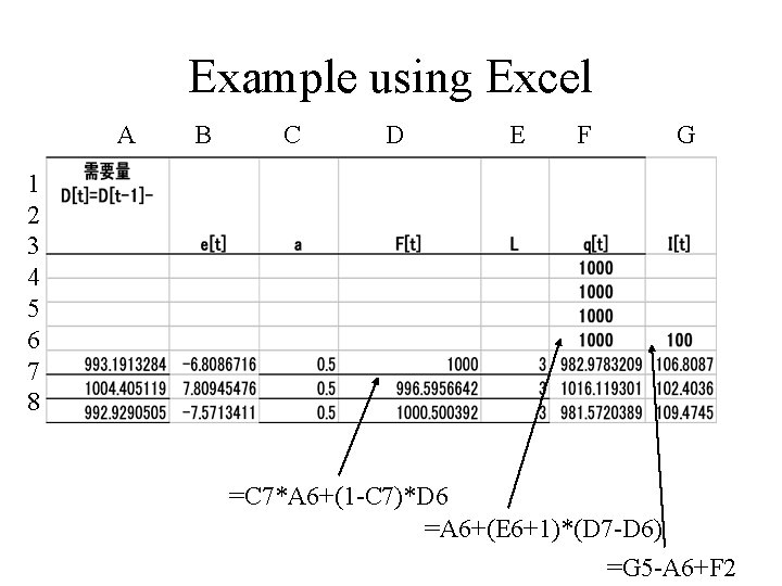
Example using Excel A B C D E F G 1 2 3 4 5 6 7 8 =C 7*A 6+(1 -C 7)*D 6 =A 6+(E 6+1)*(D 7 -D 6) =G 5 -A 6+F 2

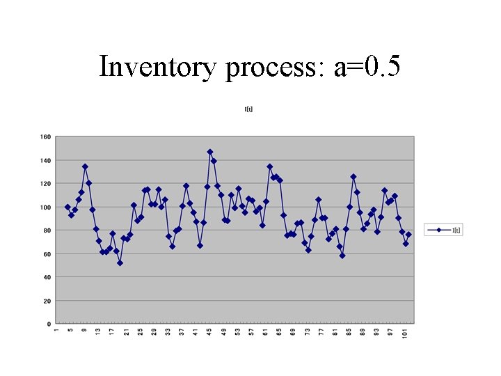
Inventory process: a=0. 5

Relationship between demand forecast

Expansion of demand forecast

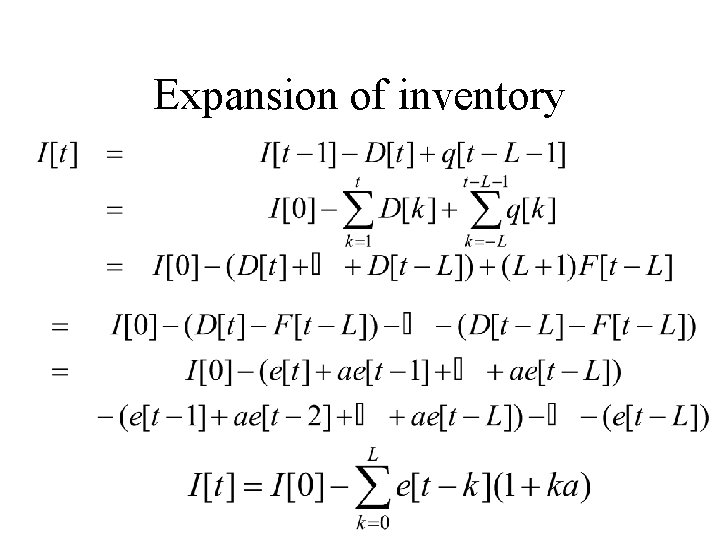
Expansion of inventory

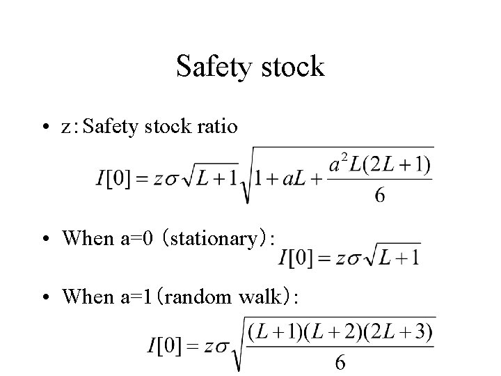
Derived formula • e[t]： mean =０，S. D. =σ, normal distribution • Expected value of inventory • Standard deviation

Safety stock • z：Safety stock ratio • When a=0 （stationary）: • When a=1（random walk）:

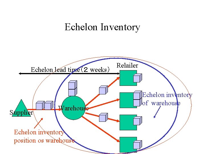
Echelon Inventory Echelon lead time（２ weeks） Supplier Warehouse Echelon inventory position os warehouse Relailer Echelon inventory of warehouse

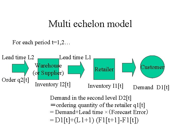
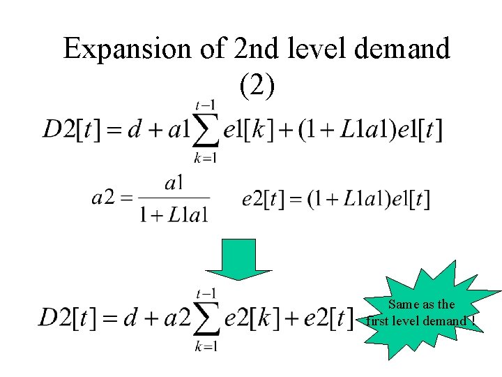
Multi echelon model For each period t=1, 2… Lead time L 2 Lead time L 1 Warehouse Retailer (or Supplier) Order q 2[t] Inventory I 1[t] Customer Demand D 1[t] Demand in the second level D 2[t] ＝ordering quantity of the retailer q 1[t] = Demand+Lead time ×（Forecast Error） = D 1[t]+(L 1+1) (F 1[t+1]-F 1[t])

Expansion of 2 nd level demand (1) D 2[t]=D 1[t]+(L 1+1) (F 1[t+1]-F 1[t])

Expansion of 2 nd level demand (2) Same as the first level demand！

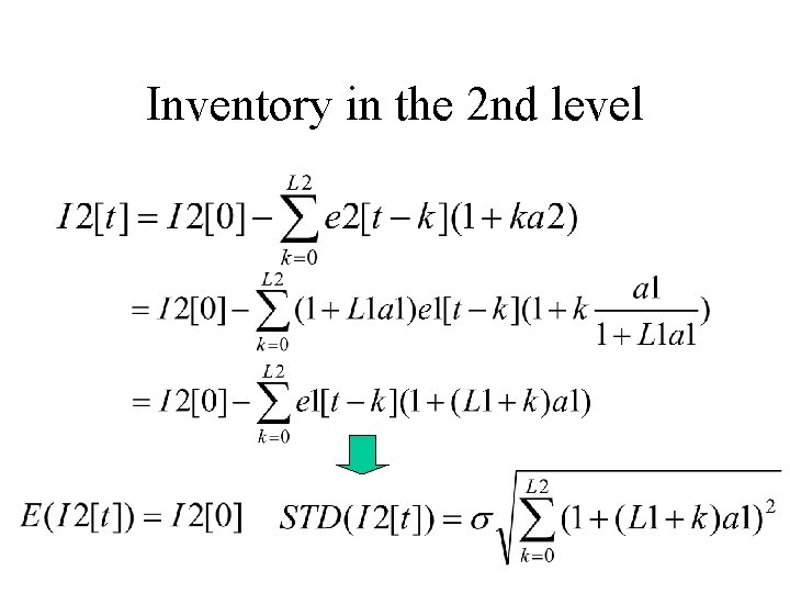
Inventory in the 2 nd level

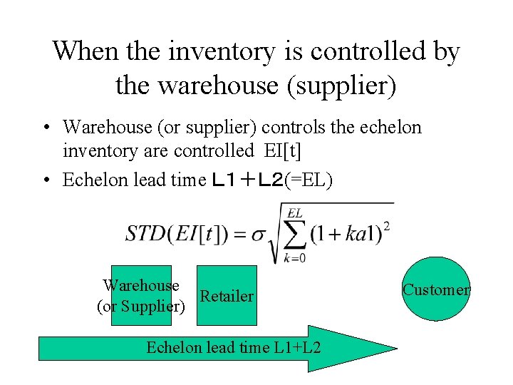
When the inventory is controlled by the warehouse (supplier) • Warehouse (or supplier) controls the echelon inventory are controlled EI[t] • Echelon lead time Ｌ１＋Ｌ２(=EL) Warehouse Retailer (or Supplier) Echelon lead time L 1+L 2 Customer

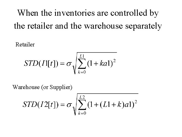
When the inventories are controlled by the retailer and the warehouse separately Retailer Warehouse (or Supplier)