Chapter 3 Inventory Management and Risk Pooling Outline

Chapter 3 Inventory Management and Risk Pooling

Outline of the contents 結束 Introduction to Inventory Management The Effect of Demand Uncertainty Ø (s, S) Policy Ø Periodic Review Policy Ø Supply Contracts Ø Risk Pooling Centralized vs. Decentralized Systems Practical Issues in Inventory Management 2

Inventory 結束 Where do we hold inventory? Ø Suppliers and manufacturers Ø Warehouses and distribution centers Ø Retailers Types of Inventory Ø Raw materials Ø WIP Ø Finished goods Why do we hold inventory? Ø Economies of scale Ø Uncertainty in supply and demand Ø Lead Time, Capacity limitations 3

Inventory 結束 Managing inventory in complex supply chains is typically difficult, and may have a significant impact on the customer service level and supply chain systemwide cost. Inventory in three types Ø Raw material inventory (where? ) Ø Work-in-process inventory (where? ) Ø Finished product inventory (where? ) 4

Why hold Inventory? 結束 Unexpected changes in customer demand. Ø The short life cycle of an increasing number of products. Thus, historical data may not be available or may be quite limited. Ø The presence of many competing products in the marketplace. (Discussed in Chapters 5 and 9) The presence in many situations of a significant uncertainty in the quantity and quality of the supply, supplier costs, and delivery times. A need to hold inventory due to delivery lead times – even if there is no uncertainty in supply or demand. Economies of scale offered by transportation companies that encourage firms to transport large quantities of items, and therefore hold large inventories. 5

Managing inventory – examples 結束 By effectively managing inventory: ØXerox eliminated $700 million inventory from its supply chain. ØWal-Mart became the largest retail company utilizing efficient inventory management. ØGM has reduced parts inventory and transportation costs by 26% annually. 6

Managing inventory – examples 結束 By not managing inventory successfully Ø In 1993, Dell’s stock plunged after the company predicted a loss. (sharply off in its forecast of demand) Ø In 1994, “IBM continues to struggle with shortages in their Think. Pad line” (WSJ, Oct 7, 1994) Ø In 1993, “Liz Claiborne said its unexpected earning decline is the consequence of higher than anticipated excess inventory” (WSJ, July 15, 1993) Ø In 2001, Cisco took a $2. 25 B excess inventory charge due to declining scales. 7

Two important issues in inventory management Demand forecasting ØForecast demand is a critical element in 結束 determining order quantity. ØWhat is the relationship between forecast demand the optimal order quantity? ØShould the order quantity “=“ or “>” or “<“ the forecast demand? Ø…. . Order quantity calculation 8

A single warehouse inventory example

Key factors affecting inventory policy? 結束 Customer demand Ø Known in advance or may be random (forecasting tools can be used). Replenishment lead time Ø May be known at the time we place the order or may be uncertain. The number of different products Ø High-mix and low volume? The length of the planning horizon 10

Key factors affecting inventory policy? 結束 Costs (order cost and inventory holding cost) Ø Order cost: the cost of the product and the transportation cost Ø Inventory holding cost üState taxes, property taxes, and insurance on inventories üMaintenance costs üObsolescence cost (an item will lose some of its value because of changes in the market. ) üOpportunities costs (the return on investment that one would receive had money been invested in something else (e. g. stock market) instead of inventory. 11

Key factors affecting inventory policy? Service level requirements ØIt is not possible to meat customer orders 100 結束 percent of the time. Managements need to specify an acceptable level of service 12

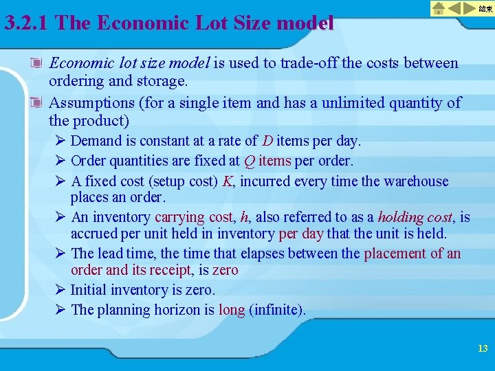
3. 2. 1 The Economic Lot Size model 結束 Economic lot size model is used to trade-off the costs between ordering and storage. Assumptions (for a single item and has a unlimited quantity of the product) Ø Demand is constant at a rate of D items per day. Ø Order quantities are fixed at Q items per order. Ø A fixed cost (setup cost) K, incurred every time the warehouse places an order. Ø An inventory carrying cost, h, also referred to as a holding cost, is accrued per unit held in inventory per day that the unit is held. Ø The lead time, the time that elapses between the placement of an order and its receipt, is zero Ø Initial inventory is zero. Ø The planning horizon is long (infinite). 13

3. 2. 1 The Economic Lot Size model 結束 Goal Ø Find the optimal order policy that minimizes annual purchasing and carrying costs while meeting all demand. Realistic system? Ø A known fixed demand over a long horizon is clear unrealistic. Ø This model will help us to develop inventory policies that are effective for more complex realistic systems. 14

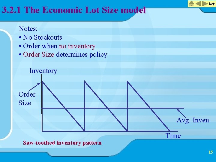
結束 3. 2. 1 The Economic Lot Size model Notes: • No Stockouts • Order when no inventory • Order Size determines policy Inventory Order Size Avg. Inven Saw-toothed inventory pattern Time 15

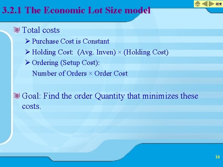
3. 2. 1 The Economic Lot Size model 結束 Total costs Ø Purchase Cost is Constant Ø Holding Cost: (Avg. Inven) × (Holding Cost) Ø Ordering (Setup Cost): Number of Orders × Order Cost Goal: Find the order Quantity that minimizes these costs. 16

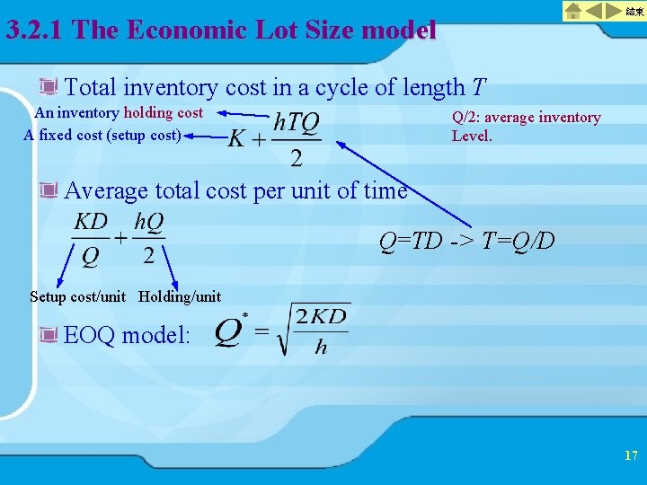
結束 3. 2. 1 The Economic Lot Size model Total inventory cost in a cycle of length T An inventory holding cost A fixed cost (setup cost) Q/2: average inventory Level. Average total cost per unit of time Q=TD -> T=Q/D Setup cost/unit Holding/unit EOQ model: 17

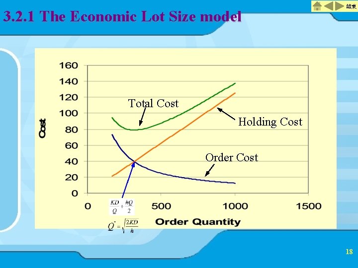
3. 2. 1 The Economic Lot Size model 結束 Total Cost Holding Cost Order Cost 18

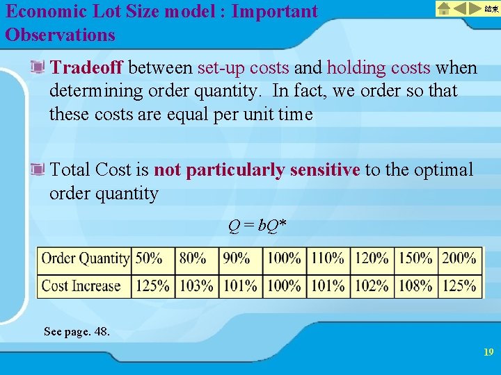
Economic Lot Size model : Important Observations 結束 Tradeoff between set-up costs and holding costs when determining order quantity. In fact, we order so that these costs are equal per unit time Total Cost is not particularly sensitive to the optimal order quantity Q = b. Q* See page. 48. 19

The Effect of Demand Uncertainty 結束 Most companies treat the world as if it were predictable: Ø Production and inventory planning are based on forecasts of demand made far in advance of the selling season Ø Companies are aware of demand uncertainty when they create a forecast, but they design their planning process as if the forecast truly represents reality Recent technological advances have increased the level of demand uncertainty: Ø Short product life cycles Ø Increasing product variety 20

Demand Forecasts 結束 The three principles of all forecasting techniques: ØForecasting is always wrong ØThe longer the forecast horizon the worst is the forecast ØAggregate forecasts are more accurate 21

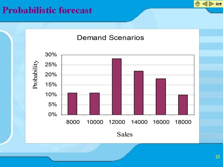
Swimsuit production 結束 (Read the case on page 49) Fashion items have short life cycles, high variety of competitors Swimsuit Ø New designs are completed Ø One production opportunity Ø Based on past sales, knowledge of the industry, and economic conditions, the marketing department has a probabilistic forecast Ø The forecast averages about 13, 000, but there is a chance that demand will be greater or less than this. 22

Probabilistic forecast 結束 23

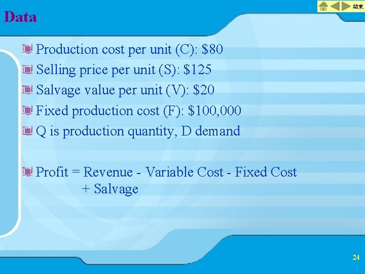
Data 結束 Production cost per unit (C): $80 Selling price per unit (S): $125 Salvage value per unit (V): $20 Fixed production cost (F): $100, 000 Q is production quantity, D demand Profit = Revenue - Variable Cost - Fixed Cost + Salvage 24

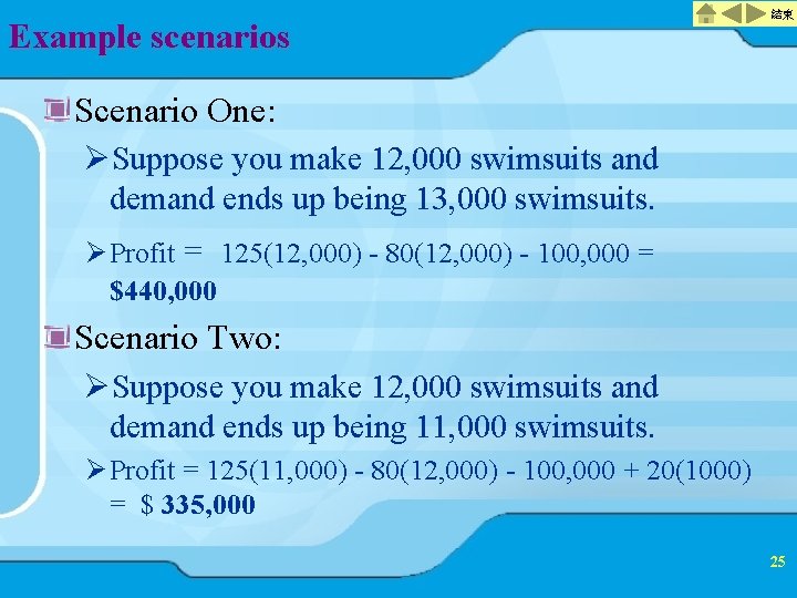
Example scenarios 結束 Scenario One: ØSuppose you make 12, 000 swimsuits and demand ends up being 13, 000 swimsuits. Ø Profit = 125(12, 000) - 80(12, 000) - 100, 000 = $440, 000 Scenario Two: ØSuppose you make 12, 000 swimsuits and demand ends up being 11, 000 swimsuits. Ø Profit = 125(11, 000) - 80(12, 000) - 100, 000 + 20(1000) = $ 335, 000 25

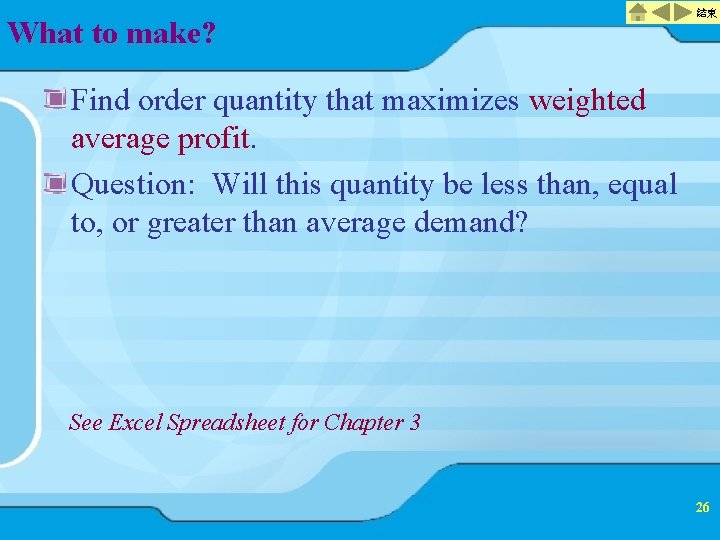
What to make? 結束 Find order quantity that maximizes weighted average profit. Question: Will this quantity be less than, equal to, or greater than average demand? See Excel Spreadsheet for Chapter 3 26

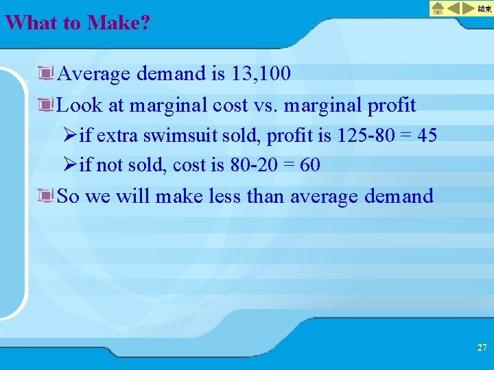
What to Make? 結束 Average demand is 13, 100 Look at marginal cost vs. marginal profit Øif extra swimsuit sold, profit is 125 -80 = 45 Øif not sold, cost is 80 -20 = 60 So we will make less than average demand 27

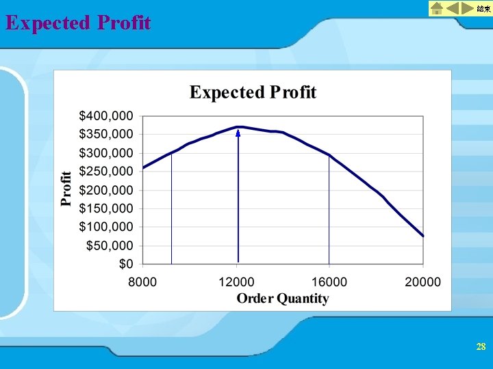
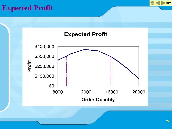
Expected Profit 結束 28

Expected Profit 結束 29

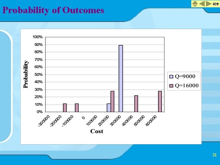
Important Observations 結束 Tradeoff between ordering enough to meet demand ordering too much Several quantities have the same average profit Average profit does not tell the whole story Question: 9000 and 16000 units lead to about the same average profit, so which do we prefer? 30

Probability of Outcomes 結束 31

Key Points from this case study 結束 The optimal order quantity is not necessarily equal to average forecast demand The optimal quantity depends on the relationship between marginal profit and marginal cost As order quantity increases, average profit first increases and then decreases As production quantity increases, risk increases. In other words, the probability of large gains and of large losses increases 32

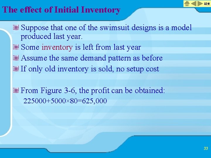
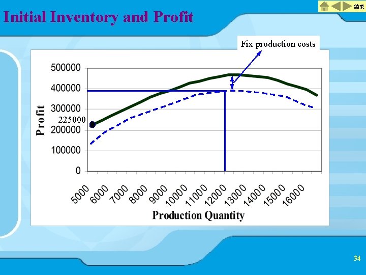
The effect of Initial Inventory 結束 Suppose that one of the swimsuit designs is a model produced last year. Some inventory is left from last year Assume the same demand pattern as before If only old inventory is sold, no setup cost From Figure 3 -6, the profit can be obtained: 225000+5000× 80=625, 000 33

結束 Initial Inventory and Profit Fix production costs 225000 34

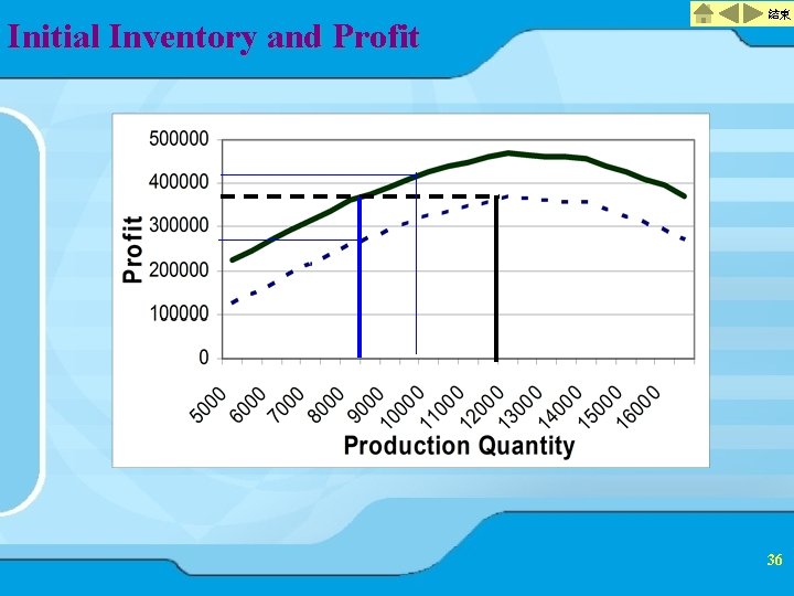
Questions 結束 If there are 7000 units remaining, what should the company do? What should they do if there are 10, 000 remaining? 35

Initial Inventory and Profit 結束 36

(s, S) Policies 結束 For some starting inventory levels, it is better to not start production If we start, we always produce to the same level Thus, we use an (s, S) policy. If the inventory level is below s, we produce up to S. s is the reorder point, and S is the order-up-to level The difference between the two levels is driven by the fixed costs associated with ordering, transportation, or manufacturing Swimsuit case: s = 8, 500 and S = 12, 000 37

Supply contracts 結束 In as supply contract, the buyer and supplier may agree on: Ø Pricing and volume discounts Ø Maximum and minimum purchase quantities Ø Delivery lead times Ø Product or material quality Ø Product return policies Refer to the Excel spreadsheet (supply contract). 38

Swimsuit example again 結束 (Read the case of example 3 -2 on page 53) Sequential supply chain: Ø each party determines its own course of action independent of the other parties. Ø For the earlier example, the retailer assumes all of the risk, of having more inventory than sales, while the manufacturer takes no risk. Ø Larger the order is, better it is for the manufacturer but it has a reverse impact to the retailer. 39

Buy-back contracts 結束 In a buy-back contract, the seller agrees to buy back unsold goods from the buyer for some agreed-upon price. Study example 3 -3 on page 54 and explain how does it work? 40

Revenue-sharing contracts 結束 For the swimsuit example, if the manufacturer is willing to give discounts, the retailer will have an incentive to order more. Study example 3 -4 and explain how does it works. 41

Quantity-flexibility contracts 結束 The supplier provides full unsold items as long as the number of returns is no larger than a certain quantity. How is it different from buy-back contracts? 42

Sales rebate contracts 結束 Sales rebate (discounts) contacts provide a direct incentive to the retailer to increase sales by means of a rebate paid by the supplier for any item sold above a certain quantity. 43

Global optimization 結束 What is the best strategy for the entire supply chain? The difficulty with global optimization is that it requires the firm to surrender decision-making power to an unbiased decision maker. See example 3 -5 on page 56 Its main drawback is that it does not provide a mechanism to allocate supply chain profit between the partners. See example 3 -6 on page 57 44

Multiple reorder opportunities 結束 Consider a central distribution facility which orders from a manufacturer and delivers to retailers. The distributor periodically places orders to replenish its inventory Continuous review policy and periodic review policy 45

The Multi-Period Inventory Model 結束 Normally distributed random demand Fixed order cost plus a cost proportional to amount ordered. Inventory cost is charged per item per unit time If an order arrives and there is no inventory, the order is lost The distributor has a required service level. This is expressed as the likelihood that the distributor will not stock out during lead time. Intuitively, what will a good policy look like? 46

Continuous review policy 結束 Known parameters Ø AVG = average daily demand faced by the distributor Ø STD = Standard deviation of daily demand faced by the distributor Ø L = Replenishment lead time from the supplier to the distributor in days Ø h = Cost of holding one unit of the product for one day at the distributor Ø = service level 47

Continuous review policy 結束 Inventory position: Ø The actual inventory at the warehouse plus items ordered by the distributor that have not yet arrived minus items that are backordered. 48

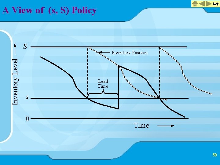
The (s, S) Policy 結束 (s, S) Policy: Whenever the inventory position drops below a certain level, s, we order to raise the inventory position to level S. The reorder point is a function of: Ø The Lead Time Ø Average demand Ø Demand variability Ø Service level 49

結束 A View of (s, S) Policy Inventory Level S Inventory Position Lead Time s 0 Time 50

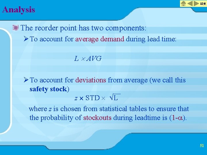
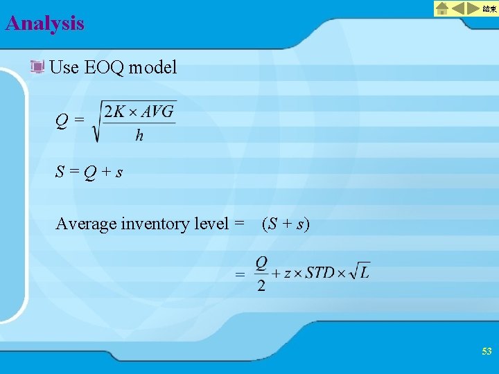
結束 Analysis The reorder point has two components: Ø To account for average demand during lead time: L AVG Ø To account for deviations from average (we call this safety stock) z STD L where z is chosen from statistical tables to ensure that the probability of stockouts during leadtime is (1 - ). 51

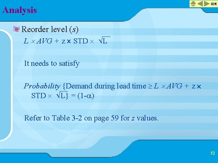
Analysis 結束 Reorder level (s) L AVG + z STD L It needs to satisfy Probability {Demand during lead time L AVG + z STD L} = (1 - ) Refer to Table 3 -2 on page 59 for z values. 52

結束 Analysis Use EOQ model Q= S=Q+s Average inventory level = (S + s) = 53

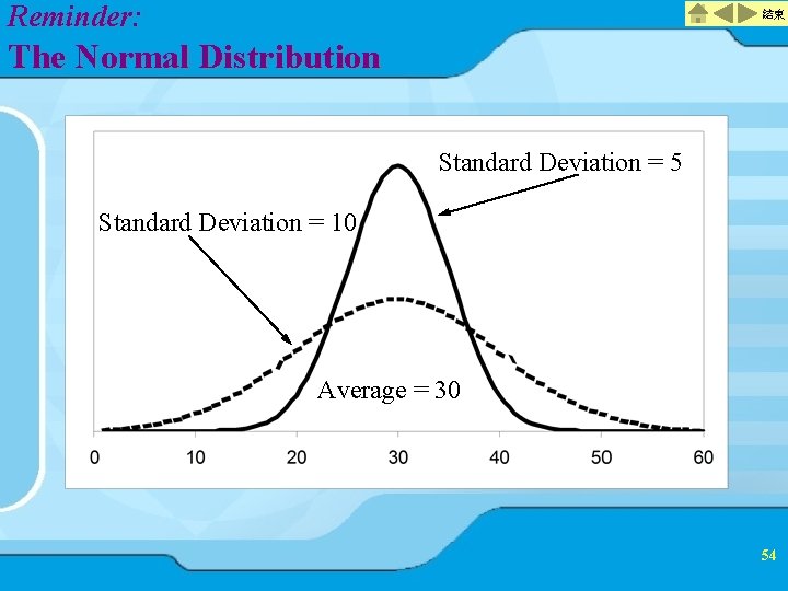
Reminder: 結束 The Normal Distribution Standard Deviation = 5 Standard Deviation = 10 Average = 30 54

The distributor holds inventory to: 結束 Satisfy demand during lead time Protect against demand uncertainty Balance fixed costs and holding costs 55

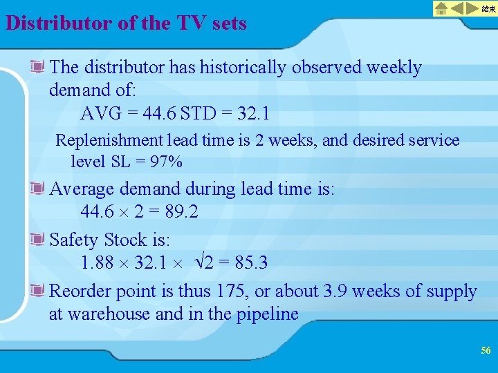
Distributor of the TV sets 結束 The distributor has historically observed weekly demand of: AVG = 44. 6 STD = 32. 1 Replenishment lead time is 2 weeks, and desired service level SL = 97% Average demand during lead time is: 44. 6 2 = 89. 2 Safety Stock is: 1. 88 32. 1 2 = 85. 3 Reorder point is thus 175, or about 3. 9 weeks of supply at warehouse and in the pipeline 56

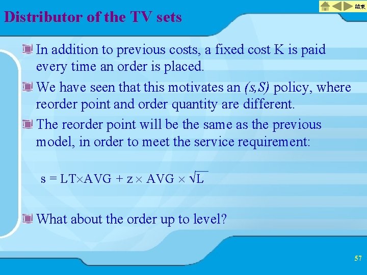
Distributor of the TV sets 結束 In addition to previous costs, a fixed cost K is paid every time an order is placed. We have seen that this motivates an (s, S) policy, where reorder point and order quantity are different. The reorder point will be the same as the previous model, in order to meet the service requirement: s = LT AVG + z AVG L What about the order up to level? 57

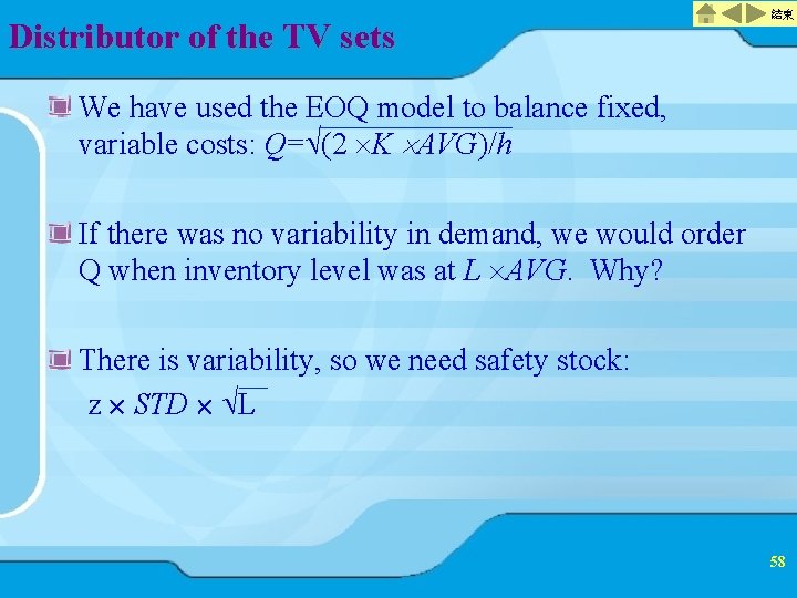
Distributor of the TV sets 結束 We have used the EOQ model to balance fixed, variable costs: Q= (2 K AVG)/h If there was no variability in demand, we would order Q when inventory level was at L AVG. Why? There is variability, so we need safety stock: z STD L 58

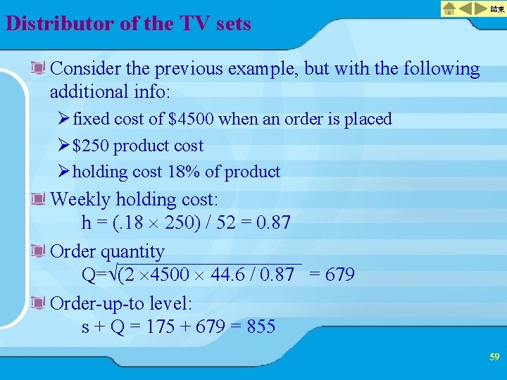
Distributor of the TV sets 結束 Consider the previous example, but with the following additional info: Ø fixed cost of $4500 when an order is placed Ø $250 product cost Ø holding cost 18% of product Weekly holding cost: h = (. 18 250) / 52 = 0. 87 Order quantity Q= (2 4500 44. 6 / 0. 87 = 679 Order-up-to level: s + Q = 175 + 679 = 855 59

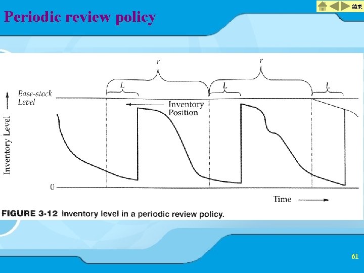
Periodic review policy 結束 Base-stock level ØEach review period, the inventory position is reviewed and the warehouse orders enough to raise the inventory position to the base-stock level. Assume that orders are placed every r period of time. 60

Periodic review policy 結束 61

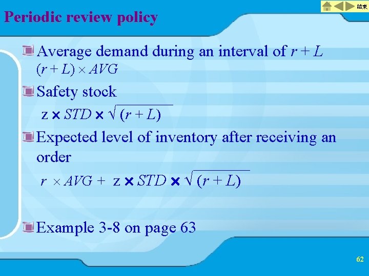
Periodic review policy 結束 Average demand during an interval of r + L (r + L) AVG Safety stock z STD (r + L) Expected level of inventory after receiving an order r AVG + z STD (r + L) Example 3 -8 on page 63 62

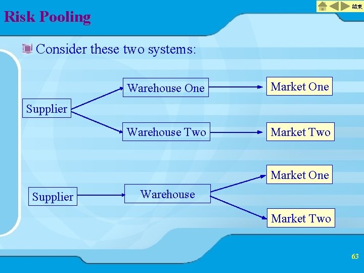
結束 Risk Pooling Consider these two systems: Warehouse One Market One Warehouse Two Market Two Supplier Market One Supplier Warehouse Market Two 63

Risk Pooling 結束 For the same service level, which system will require more inventory? Why? For the same total inventory level, which system will have better service? Why? What are the factors that affect these answers? 64

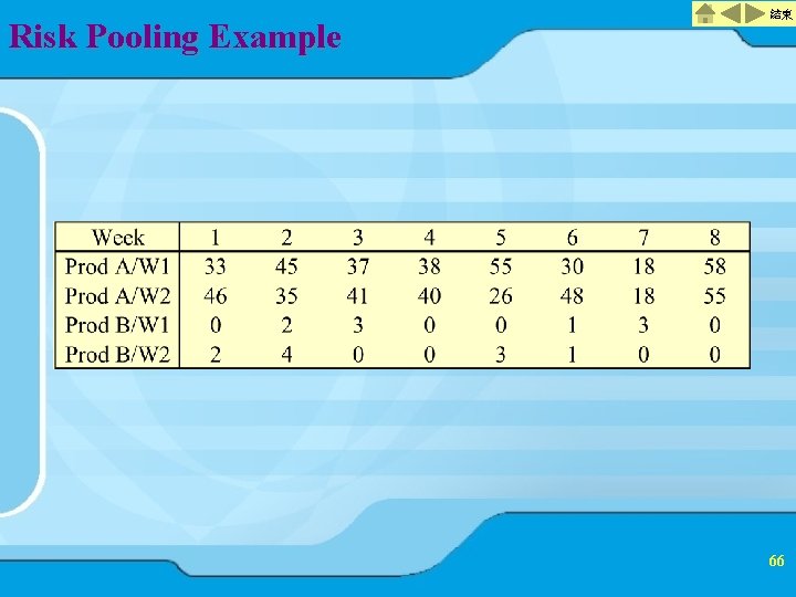
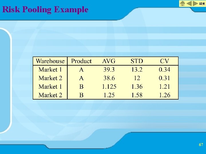
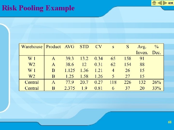
Risk Pooling Example 結束 Compare the two systems: (Read the case on page. 6466) Ø two products Ø maintain 97% service level Ø $60 order cost Ø $. 27 weekly holding cost Ø $1. 05 transportation cost per unit in decentralized system, $1. 10 in centralized system Ø 1 week lead time 65

Risk Pooling Example 結束 66

Risk Pooling Example 結束 67

Risk Pooling Example 結束 68

Risk Pooling: Important Observations 結束 Centralizing inventory control reduces both safety stock and average inventory level for the same service level. This works best for Ø High coefficient of variation, which reduces required safety stock. Ø Negatively correlated demand. Why? What other kinds of risk pooling will we see? 69

結束 Risk Pooling: Types of Risk Pooling Across Markets Risk Pooling Across Products Risk Pooling Across Time Ø Daily order up to quantity is: üLT AVG + z AVG L Orders 10 11 12 13 14 15 Demands 70

To Centralize or not to Centralize 結束 Safety stock Ø Safety stock decreases as a firm moves from a decentralized to a centralized system. Ø Depend on CV and correlation Service level Ø Given the same total safety stock, the service level provided by the centralized system is higher. Overhead Ø Typically, these costs are much greater in a decentralized system. 71

To Centralize or not to Centralize 結束 Lead time ØThe response time for a decentralized system is much shorter. Transportation Costs ØOutbound costs are higher for the centralized system. ØInbound costs are higher for the decentralized system. 72

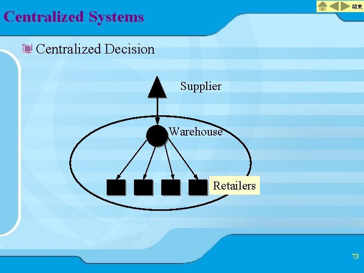
結束 Centralized Systems Centralized Decision Supplier Warehouse Retailers 73

Centralized Distribution Systems 結束 Question: How much inventory should management keep at each location? A good strategy: Ø The retailer raises inventory to level s each period Ø The supplier raises the sum of inventory in the retailer and supplier warehouses and in transit to S Ø If there is not enough inventory in the warehouse to meet all demands from retailers, it is allocated so that the service level at each of the retailers will be equal. 74

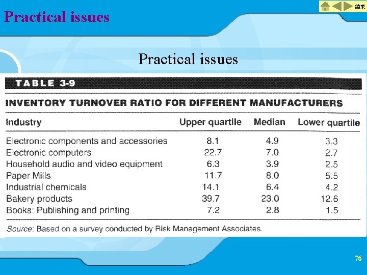
Practical issues 結束 Periodic inventory review policy Tight management of usage rates, lead times and safety stock Reduced safety stock levels Introduce or enhance cycle counting practice ABC approach Shift more inventory, or inventory ownership, to suppliers Quantitative approaches – inventory turnover rate 75

結束 Practical issues 76

Forecasting 結束 Three rules of forecasting ØThe forecast is always wrong. ØThe longer the forecast horizon, the worse the forecast. ØAggregate forecasts are more accurate. 77

Forecasting 結束 Categories (See section 3. 7) ØJudgment methods ØMarket research methods ØTime-series methods ØCausal methods 78

Summary 結束 Matching supply and demand in the supply chain is a critical challenge. ØUnfortunately, the existence three forecasting rules. Globally optimal inventory policies, in which the best possible policy for the entire supply chain is implemented, are the best course of action. Well-designed supply contracts frequently make this global optimization possible. 79