Independent Demand Inventory Systems 1 Inventory Inventory a

Independent Demand Inventory Systems 1

Inventory • Inventory: a store of goods held for future use • Types of inventory: raw materials, work-in- process, finished goods, and supplies (MRO) • Importance: among some firms, inventory carrying costs represent from 10 to 40 percent of the cost of goods sold 2

Why Hold Inventory? 1. 2. 3. 4. 5. 6. 7. 8. 9. Meet expected customer demand Improve customer service Uncertain sources of supply Economies of scale Stable (smooth) rates of production An inability to backlog demand Decouple operations Forward buying Display items 3

Independent Demand Versus Dependent Demand • An important distinction between independent and dependent demand • Independent demand inventory control procedures rely upon unbiased forecasts of uncertain demand. Demand lead times may be treated as random variables. Forecasts are used to develop production and purchase schedules for end items. • Dependent demand inventory control procedures rely upon the certain demand relationship in order to determine production and purchase schedules. 4

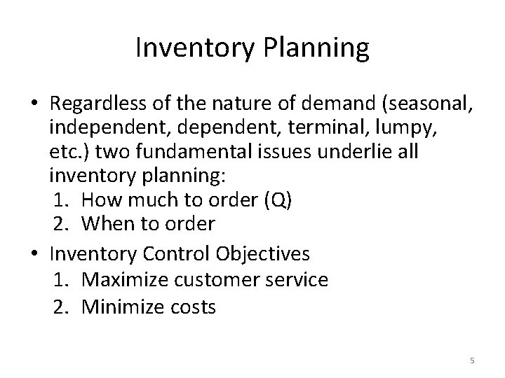
Inventory Planning • Regardless of the nature of demand (seasonal, independent, terminal, lumpy, etc. ) two fundamental issues underlie all inventory planning: 1. How much to order (Q) 2. When to order • Inventory Control Objectives 1. Maximize customer service 2. Minimize costs 5

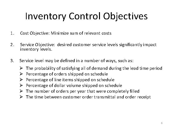
Inventory Control Objectives 1. Cost Objective: Minimize sum of relevant costs 2. Service Objective: desired customer service levels significantly impact inventory levels. 3. Service level may be defined in a number of ways, such as: Ø Ø Ø The probability of satisfying all of demand during the lead time period Percentage of orders shipped on schedule Percentage of line items shipped on schedule Percentage of dollar volume shipped on schedule The number of orders per year that were completely filled The time between customer order transmittal and order receipt 6

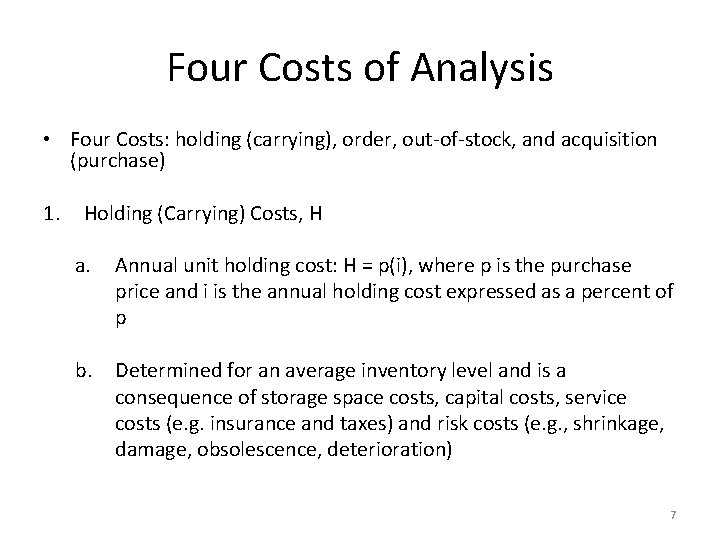
Four Costs of Analysis • Four Costs: holding (carrying), order, out-of-stock, and acquisition (purchase) 1. Holding (Carrying) Costs, H a. Annual unit holding cost: H = p(i), where p is the purchase price and i is the annual holding cost expressed as a percent of p b. Determined for an average inventory level and is a consequence of storage space costs, capital costs, service costs (e. g. insurance and taxes) and risk costs (e. g. , shrinkage, damage, obsolescence, deterioration) 7

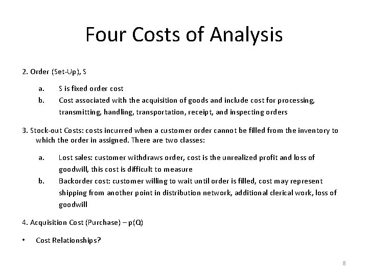
Four Costs of Analysis 2. Order (Set-Up), S a. b. S is fixed order cost Cost associated with the acquisition of goods and include cost for processing, transmitting, handling, transportation, receipt, and inspecting orders 3. Stock-out Costs: costs incurred when a customer order cannot be filled from the inventory to which the order in assigned. There are two classes: a. b. Lost sales: customer withdraws order, cost is the unrealized profit and loss of goodwill, this cost is difficult to measure Backorder cost: customer willing to wait until order is filled, cost may represent shipping from another point in distribution network, additional clerical work, loss of goodwill 4. Acquisition Cost (Purchase) – p(Q) • Cost Relationships? 8

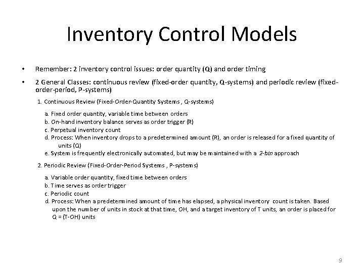
Inventory Control Models • Remember: 2 inventory control issues: order quantity (Q) and order timing • 2 General Classes: continuous review (fixed-order quantity, Q-systems) and periodic review (fixedorder-period, P-systems) 1. Continuous Review (Fixed-Order-Quantity Systems , Q-systems) a. Fixed order quantity, variable time between orders b. On-hand inventory balance serves as order trigger (R) c. Perpetual inventory count d. Process: When inventory drops to a predetermined amount (R), an order is released for a fixed quantity of units (Q) e. System is frequently electronically automated, but may be maintained with a 2 -bin approach 2. Periodic Review (Fixed-Order-Period Systems , P-systems) a. Variable order quantity, fixed time between orders b. Time serves as order trigger c. Periodic count d. Process: When a predetermined amount of time has elapsed, a physical inventory count is taken. Based upon the number of units in stock at that time, OH, and a target inventory of T units, an order is placed for Q = (T-OH) units 9

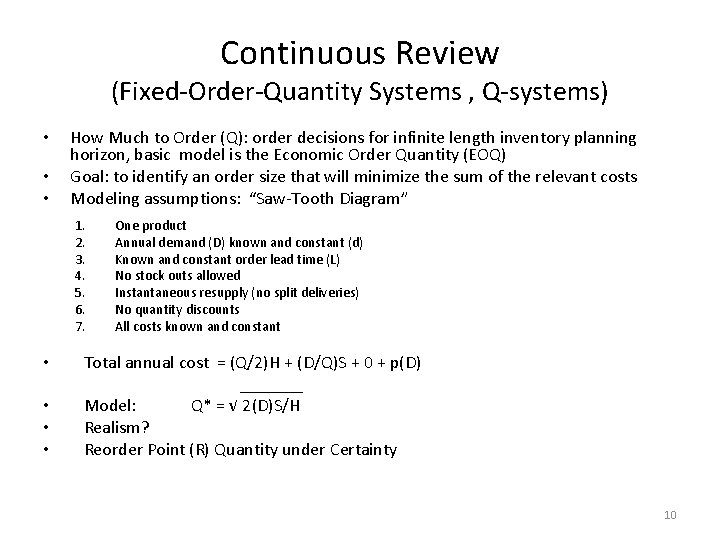
Continuous Review (Fixed-Order-Quantity Systems , Q-systems) • • • How Much to Order (Q): order decisions for infinite length inventory planning horizon, basic model is the Economic Order Quantity (EOQ) Goal: to identify an order size that will minimize the sum of the relevant costs Modeling assumptions: “Saw-Tooth Diagram” 1. 2. 3. 4. 5. 6. 7. • • One product Annual demand (D) known and constant (d) Known and constant order lead time (L) No stock outs allowed Instantaneous resupply (no split deliveries) No quantity discounts All costs known and constant Total annual cost = (Q/2)H + (D/Q)S + 0 + p(D) _______ Model: Q* = √ 2(D)S/H Realism? Reorder Point (R) Quantity under Certainty 10

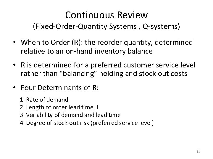
Continuous Review (Fixed-Order-Quantity Systems , Q-systems) • When to Order (R): the reorder quantity, determined relative to an on-hand inventory balance • R is determined for a preferred customer service level rather than “balancing” holding and stock out costs • Four Determinants of R: 1. Rate of demand 2. Length of order lead time, L 3. Variability of demand lead time 4. Degree of stock-out risk (preferred service level) 11

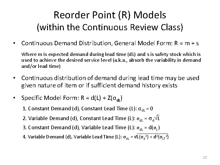
Reorder Point (R) Models (within the Continuous Review Class) • Continuous Demand Distribution, General Model Form: R = m + s Where m is expected demand during lead time (d. L) and s is safety stock which is used to achieve the desired service level (a. k. a. , absorb the variability in demand and/or lead time) • Continuous distribution of demand during lead time may be used given nature of item or if sufficient demand history exists • Specific Model Form: R = d(L) + Z(σd. L) 1. Constant Demand (d), Constant Lead Time (L): σd. L = 0 __ 2. Variable Demand (d), Constant Lead Time (L): σd. L = d L 3. Constant Demand (d), Variable Lead Time (L): σd. L = d(σL) ____________ 4. Variable Demand (d), Variable Lead Time (L): σd. L = √L(σd 2) + d 2(σLT 2) 12

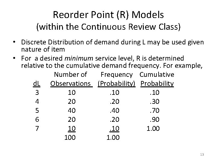
Reorder Point (R) Models (within the Continuous Review Class) • Discrete Distribution of demand during L may be used given nature of item • For a desired minimum service level, R is determined relative to the cumulative demand frequency. For example, Number of Frequency Cumulative d. L Observations (Probability) Probability 3 10 . 10 4 20 . 20 . 30 5 40 . 40 . 70 6 20 . 20 . 90 7 10 1. 00 100 1. 00 13

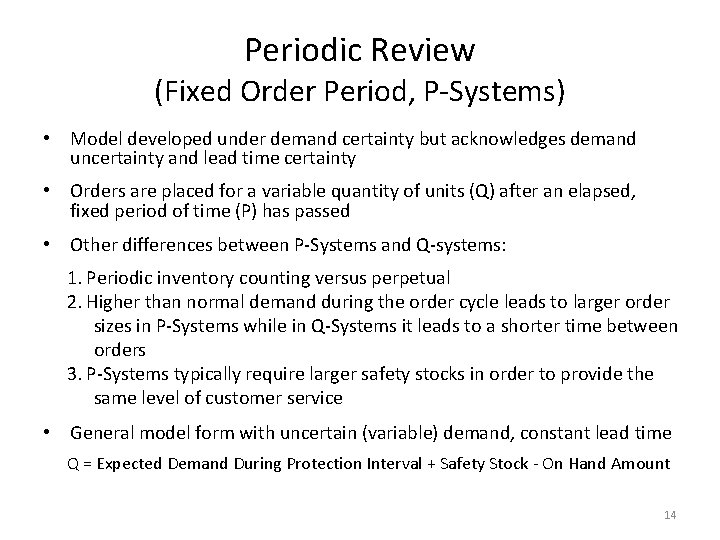
Periodic Review (Fixed Order Period, P-Systems) • Model developed under demand certainty but acknowledges demand uncertainty and lead time certainty • Orders are placed for a variable quantity of units (Q) after an elapsed, fixed period of time (P) has passed • Other differences between P-Systems and Q-systems: 1. Periodic inventory counting versus perpetual 2. Higher than normal demand during the order cycle leads to larger order sizes in P-Systems while in Q-Systems it leads to a shorter time between orders 3. P-Systems typically require larger safety stocks in order to provide the same level of customer service • General model form with uncertain (variable) demand, constant lead time Q = Expected Demand During Protection Interval + Safety Stock - On Hand Amount 14

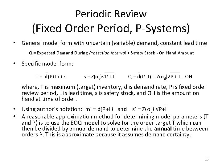
Periodic Review (Fixed Order Period, P-Systems) • General model form with uncertain (variable) demand, constant lead time Q = Expected Demand During Protection Interval + Safety Stock - On Hand Amount • Specific model form: ____ T = d(P+L) + s s = Z(σd)√P + L Q = d(P+L) + Z(σd)√P + L - OH where, T is maximum (target) inventory, d is demand rate, P is fixed order review period, L is lead time, s is safety stock, and OH is the amount on hand at time of order. _____ _ • Using author’s notation: m’ = d(P+L) and s’ = Z(σd) √P+L • A reasonable approximation method for determining model parameters (T and P) is to use the EOQ model to solve for the order target T which can then be divided by annual demand to determine the annual time between orders P. This is approximate because it assumes demand certainty. 15

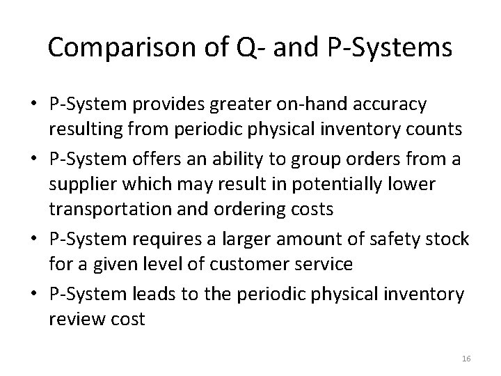
Comparison of Q- and P-Systems • P-System provides greater on-hand accuracy resulting from periodic physical inventory counts • P-System offers an ability to group orders from a supplier which may result in potentially lower transportation and ordering costs • P-System requires a larger amount of safety stock for a given level of customer service • P-System leads to the periodic physical inventory review cost 16

Additional Inventory Issues • Cycle counting: How often? • ABC Inventory Classification Schemes: How many and break points? 17