Safety Inventory Safety Inventory is inventory carried for

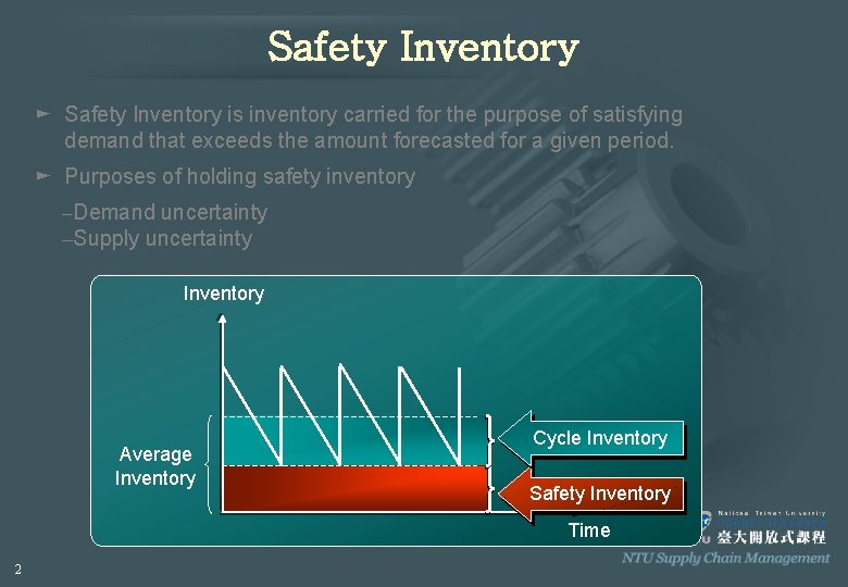
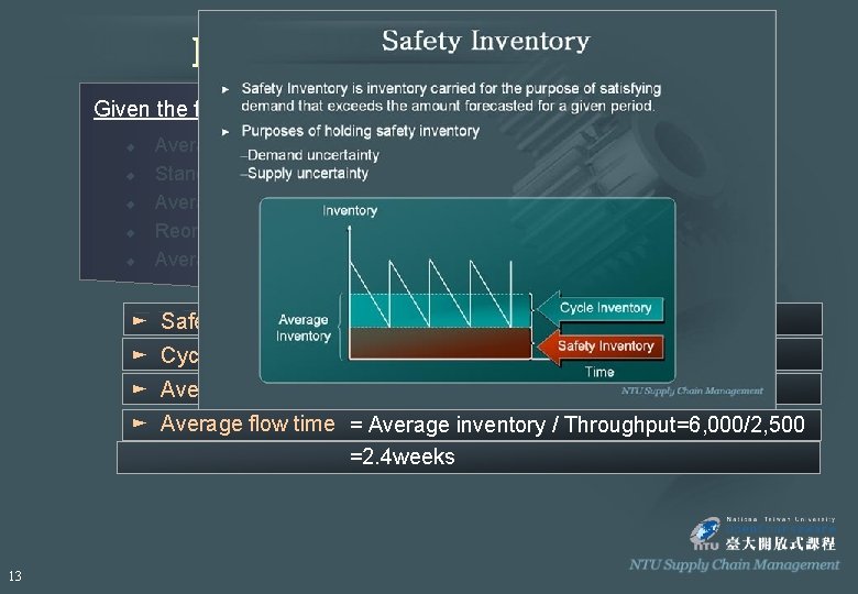
Safety Inventory ► Safety Inventory is inventory carried for the purpose of satisfying demand that exceeds the amount forecasted for a given period. ► Purposes of holding safety inventory –Demand uncertainty –Supply uncertainty Inventory Average Inventory Cycle Inventory Safety Inventory Time 2

Planning Safety Inventory ► Appropriate level of safety inventory is determined by 》 Uncertainty of both demand supply – Uncertainty increases, then safety inventory increases. 》 Desired level of product availability – increases, then safety inventory increases. ► Actions to improve product availability while reducing safety inventory 3

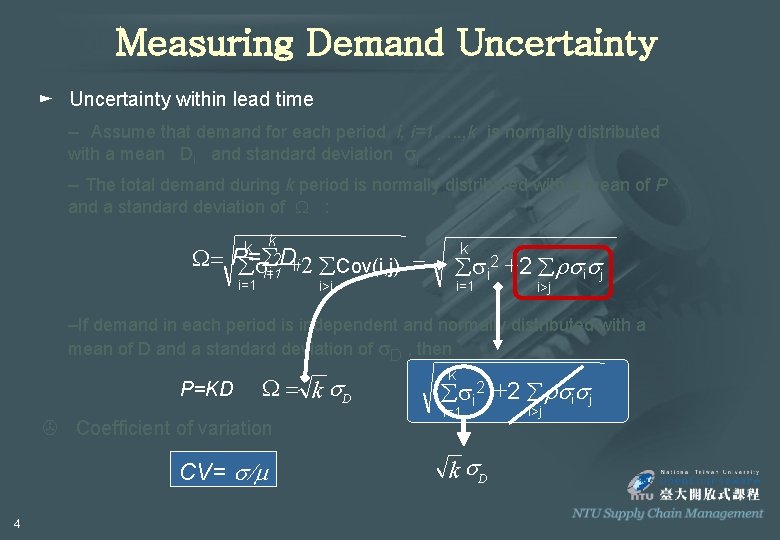
Measuring Demand Uncertainty ► Uncertainty within lead time – Assume that demand for each period i, i=1, …. , k is normally distributed with a mean Di and standard deviation si. – The total demand during k period is normally distributed with a mean of P and a standard deviation of W : W= k P= 2 Di åså i=1 i +2 k i=1 åCov(i, j) = i>j k åsi 2 +2 årsisj i=1 i>j –If demand in each period is independent and normally distributed with a mean of D and a standard deviation of s. D , then P=KD W = k s. D > Coefficient of variation CV= s/m 4 k åsi 2 +2 årsisj i=1 k s. D i>j

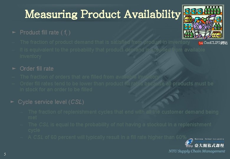
Measuring Product Availability ► Product fill rate ( fr ) Cool. CLIPS網站 – The fraction of product demand that is satisfied from product in inventory – It is equivalent to the probability that product demand is supplied from available inventory ► Order fill rate – The fraction of orders that are filled from available inventory – Order fill rates tend to be lower than product fill rates because all products must be in stock for an order to be filled ► Cycle service level (CSL) – The fraction of replenishment cycles that end with all the customer demand being met – The CSL is equal to the probability of not having a stockout in a replenishment cycle – A CSL of 60 percent will typically result in a fill rate higher than 60% 5

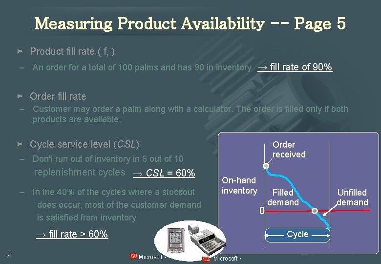
Measuring Product Availability -- Page 5 ► Product fill rate ( fr ) – An order for a total of 100 palms and has 90 in inventory → fill rate of 90% ► Order fill rate – Customer may order a palm along with a calculator. The order is filled only if both products are available. ► Cycle service level (CSL) Order received – Don't run out of inventory in 6 out of 10 replenishment cycles → CSL = 60% – In the 40% of the cycles where a stockout does occur, most of the customer demand is satisfied from inventory On-hand inventory 0 → fill rate > 60% 6 Filled demand Cycle Microsoft。 Unfilled demand

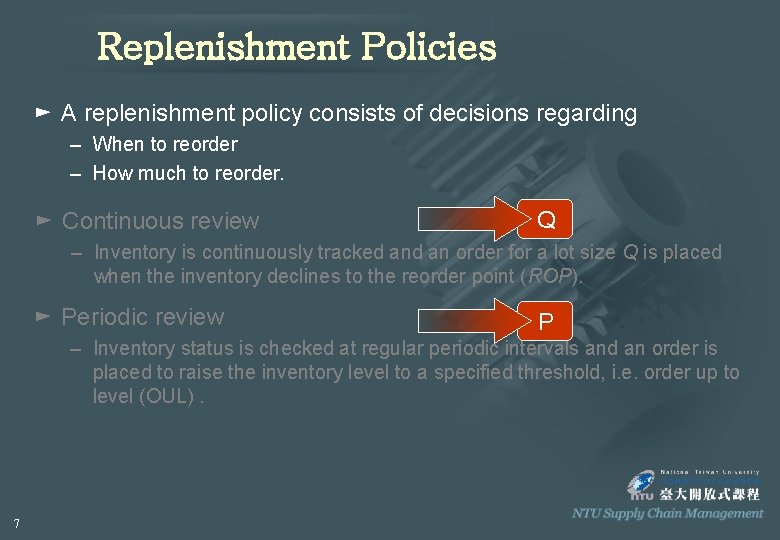
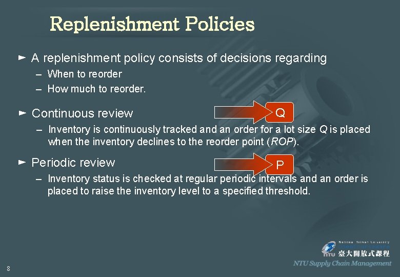
Replenishment Policies ► A replenishment policy consists of decisions regarding – When to reorder – How much to reorder. ► Continuous review Q – Inventory is continuously tracked an order for a lot size Q is placed when the inventory declines to the reorder point (ROP). ► Periodic review P – Inventory status is checked at regular periodic intervals and an order is placed to raise the inventory level to a specified threshold, i. e. order up to level (OUL). 7

Replenishment Policies ► A replenishment policy consists of decisions regarding – When to reorder – How much to reorder. ► Continuous review Q – Inventory is continuously tracked an order for a lot size Q is placed when the inventory declines to the reorder point (ROP). ► Periodic review P – Inventory status is checked at regular periodic intervals and an order is placed to raise the inventory level to a specified threshold. 8

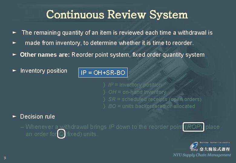
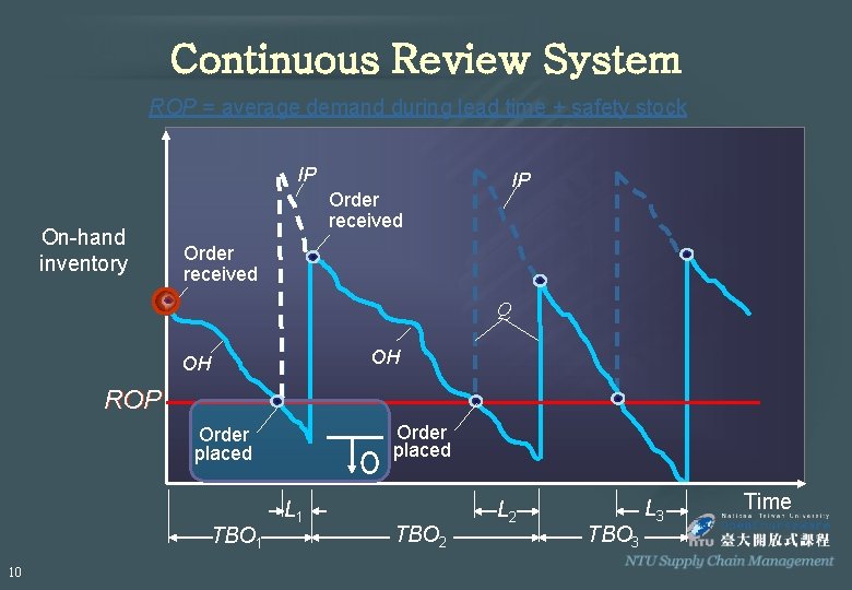
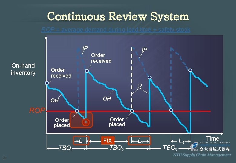
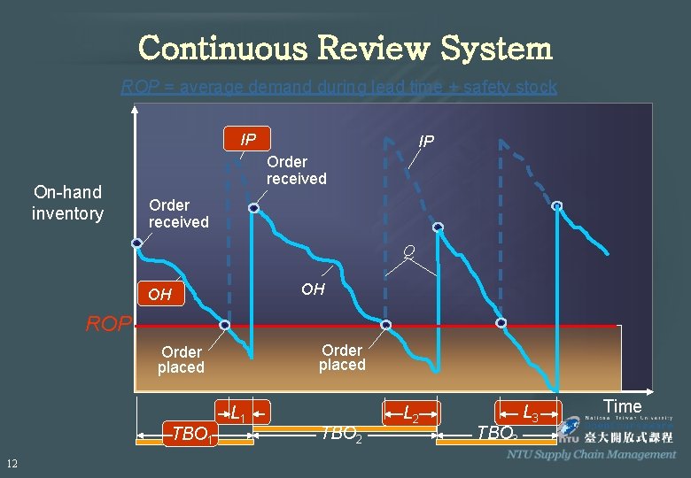
Continuous Review System ► The remaining quantity of an item is reviewed each time a withdrawal is ► made from inventory, to determine whether it is time to reorder. ► Other names are: Reorder point system, fixed order quantity system ► Inventory position IP = OH+SR-BO 》IP = inventory position 》OH = on-hand inventory 》SR = scheduled receipts (open orders) 》BO = units backordered or allocated ► Decision rule – Whenever a withdrawal brings IP down to the reorder point (ROP), place an order for Q (fixed) units. 9

Continuous Review System ROP = average demand during lead time + safety stock IP On-hand inventory IP Order received Q OH OH ROP Order placed TBO 1 10 L 1 TBO 2 L 2 TBO 3 L 3 Time

Continuous Review System ROP = average demand during lead time + safety stock IP On-hand inventory IP Order received Q OH OH ROP Order placed TBO 1 11 L 1 FIX TBO 2 L 2 TBO 3 L 3 Time

Continuous Review System ROP = average demand during lead time + safety stock IP On-hand inventory IP Order received Q OH OH ROP Order placed TBO 1 12 L 1 TBO 2 L 2 TBO 3 L 3 Time

Example Given the following data u u u Average demand per week, D = 2, 500 Standard deviation of weekly demand, s. D =500 Average lead time for replacement, L = 2 weeks Reorder point, ROP = 6, 000 Average lot size, Q = 10, 000 ► Safety inventory, ss =ROP-DL=6, 000 -5, 000=1, 000 ► Cycle inventory =Q/2=10, 000/2=5, 000 ► Average inventory =5, 000+1, 000=6, 000 ► Average flow time = Average inventory / Throughput=6, 000/2, 500 =2. 4 weeks 13

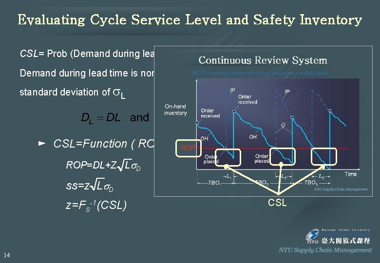
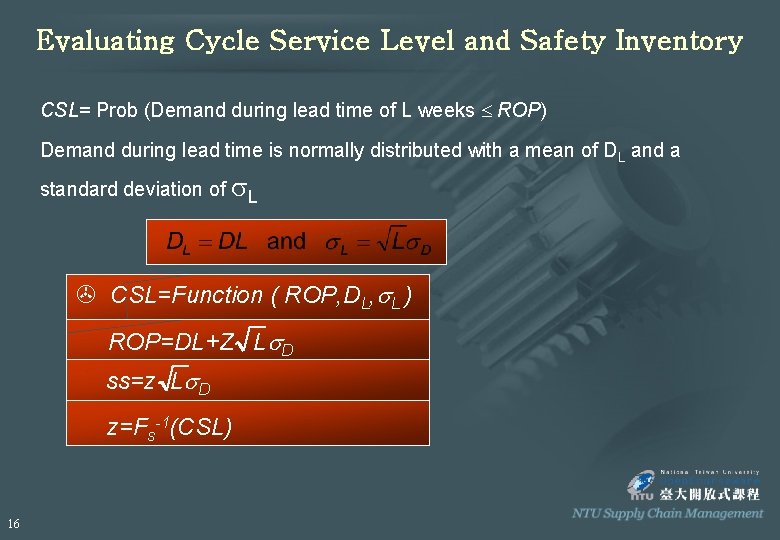
Evaluating Cycle Service Level and Safety Inventory CSL= Prob (Demand during lead time of L weeks £ ROP) Demand during lead time is normally distributed with a mean of DL and a standard deviation of s. L ► CSL=Function ( ROP, DL, s. L ) ROP=DL+Z Ls. D ss=z Ls. D z=Fs-1(CSL) 14 CSL

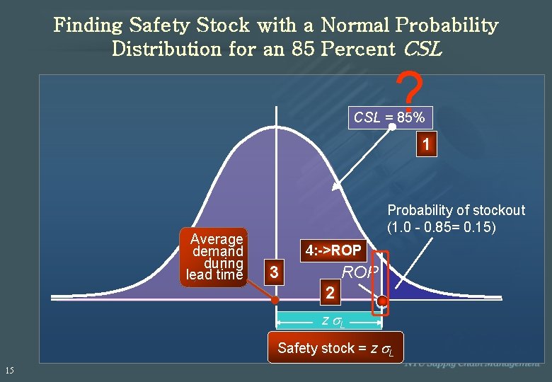
Finding Safety Stock with a Normal Probability Distribution for an 85 Percent CSL ? CSL = 85% 1 Average demand during lead time Probability of stockout (1. 0 - 0. 85= 0. 15) 4: ->ROP 3 2 z s. L Safety stock = z s. L 15

Evaluating Cycle Service Level and Safety Inventory CSL= Prob (Demand during lead time of L weeks £ ROP) Demand during lead time is normally distributed with a mean of DL and a standard deviation of s. L > CSL=Function ( ROP, DL, s. L ) ROP=DL+Z Ls. D ss=z Ls. D z=Fs-1(CSL) 16

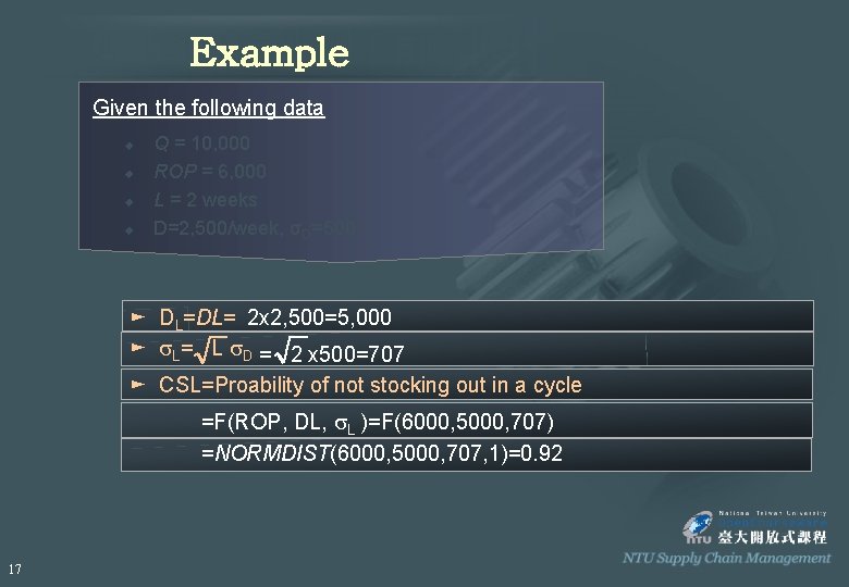
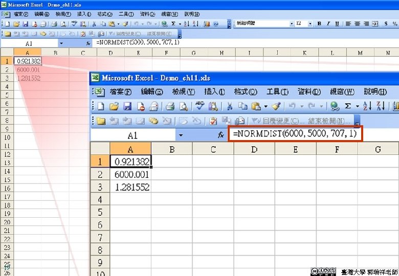
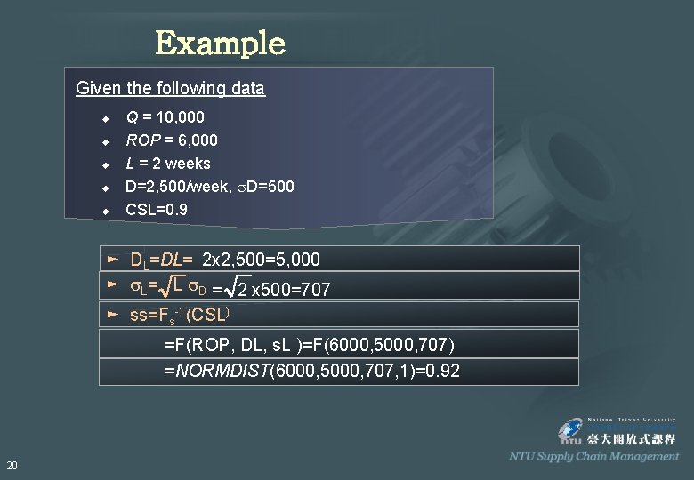
Example Given the following data u u Q = 10, 000 ROP = 6, 000 L = 2 weeks D=2, 500/week, σD=500 ► DL=DL= 2 x 2, 500=5, 000 ► s. L= L s. D = 2 x 500=707 ► CSL=Proability of not stocking out in a cycle =F(ROP, DL, s. L )=F(6000, 5000, 707) =NORMDIST(6000, 5000, 707, 1)=0. 92 17

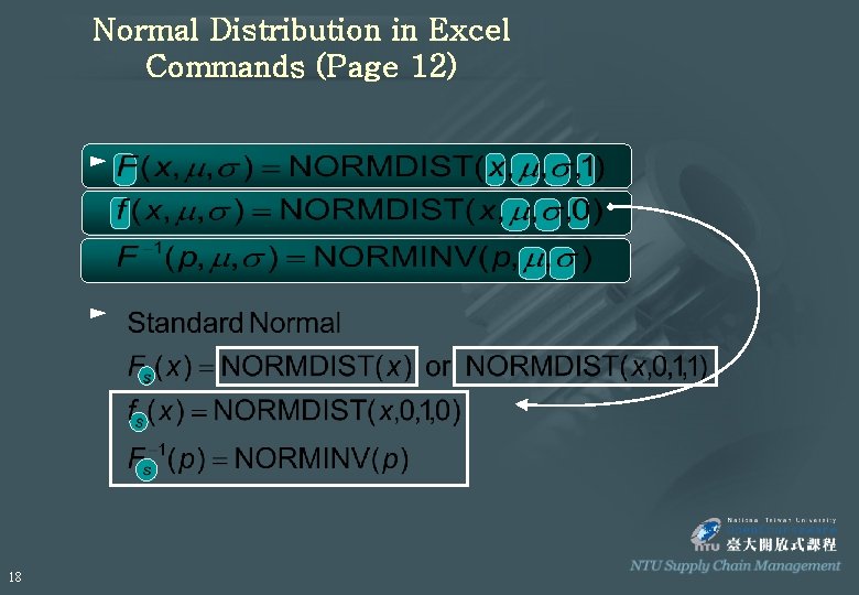
Normal Distribution in Excel Commands (Page 12) ► ► 18

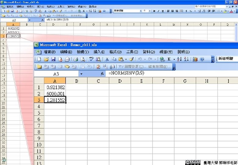
Normal Distribution in Excel (Demo) 19 臺灣大學 郭瑞祥老師

Example Given the following data u u u Q = 10, 000 ROP = 6, 000 L = 2 weeks D=2, 500/week, s. D=500 CSL=0. 9 ► DL=DL= 2 x 2, 500=5, 000 ► s. L= L s. D = 2 x 500=707 ► ss=Fs-1(CSL) =F(ROP, DL, s. L )=F(6000, 5000, 707) =NORMDIST(6000, 5000, 707, 1)=0. 92 20

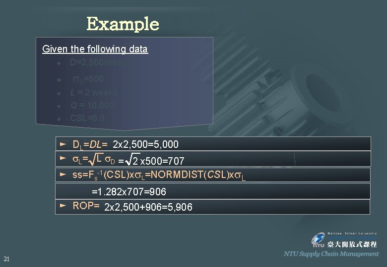
Example Given the following data u u u D=2, 500/week s. D=500 L = 2 weeks Q = 10, 000, CSL=0. 9 ► DL=DL= 2 x 2, 500=5, 000 ► s. L= L s. D = 2 x 500=707 ► ss=Fs-1(CSL)xs. L=NORMDIST(CSL)xs. L =1. 282 x 707=906 ► ROP= 2 x 2, 500+906=5, 906 21

Example Given the following data 5 D=2, 500/week 5 s. D=500 5 L = 2 weeks 5 Q = 10, 000, 5 CSL=0. 9 > DL=DL= 2 x 2, 500=5, 000 > s. L= L s. D = 2 x 500=707 > ss=Fs-1(CSL)xs. L=NORMDIST(CSL)xs. L =1. 282 x 707=906 > ROP= 2 x 2, 500+906=5, 906 22 臺灣大學 郭瑞祥老師

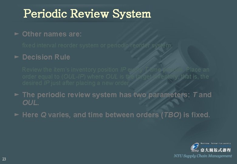
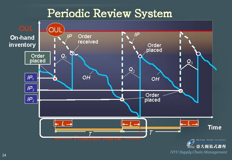
Periodic Review System ► Other names are: fixed interval reorder system or periodic reorder system. ► Decision Rule Review the item’s inventory position IP every T time periods. Place an order equal to (OUL-IP) where OUL is the target inventory, that is, the desired IP just after placing a new order. ► The periodic review system has two parameters: T and OUL. ► Here Q varies, and time between orders (TBO) is fixed. 23

Periodic Review System OUL On-hand inventory Order placed IP IP Order received Order placed Q 1 Q 3 Q 2 IP 1 OH OH IP 3 Order placed IP 2 L T Protection interval 24 L L T Time

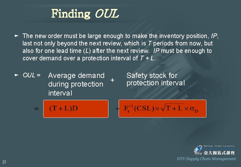
Finding OUL ► The new order must be large enough to make the inventory position, IP, last not only beyond the next review, which is T periods from now, but also for one lead time (L) after the next review. IP must be enough to cover demand over a protection interval of T + L. ► OUL = 25 Average demand + during protection interval Safety stock for protection interval

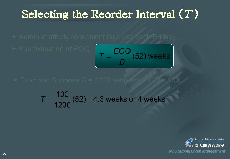
Selecting the Reorder Interval (T ) ► Administratively convenient (such as each Friday) ► Approximation of EOQ ► Example: Suppose D = 1200 /year and EOQ = 100 26

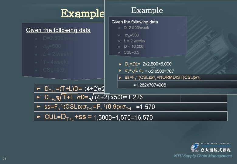
Example Given the following data u u u D=2, 500/week s. D=500 L = 2 weeks T= 4 weeks CSL=0. 9 ► DT+L=(T+L)D= (4+2)x 2, 500=15, 000 ► DT+L= T+L s. D= (4+2) x 500=1, 225 ► ss=Fs-1(CSL)xs. T+L=Fs-1(0. 9)xs. T+L =1, 570 ► OUL=DT+L+ss = 1, 5000+1, 570=16, 570 27

Periodic System versus Continuous System 28

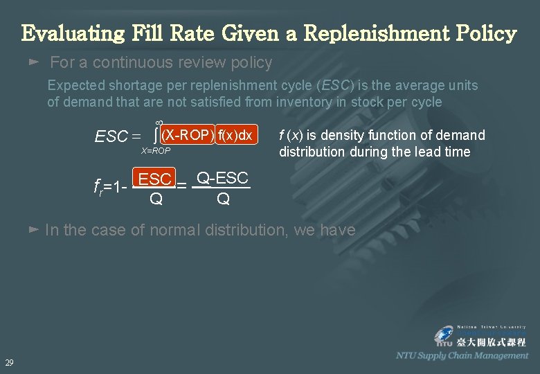
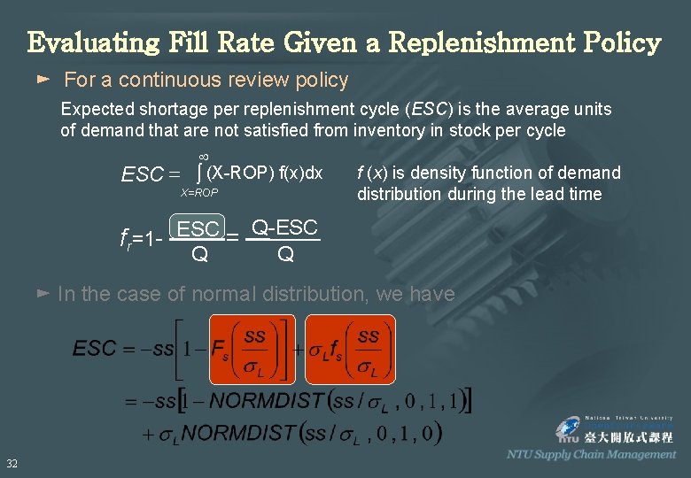
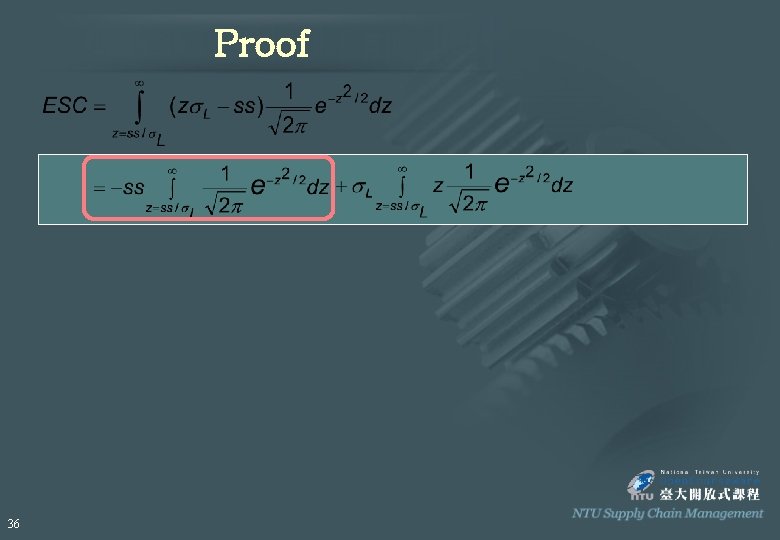
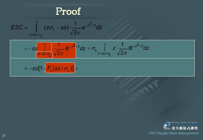
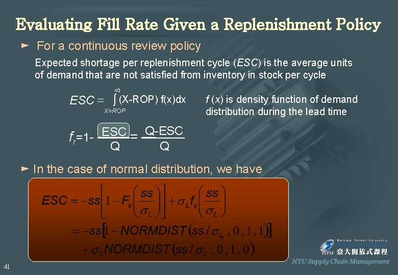
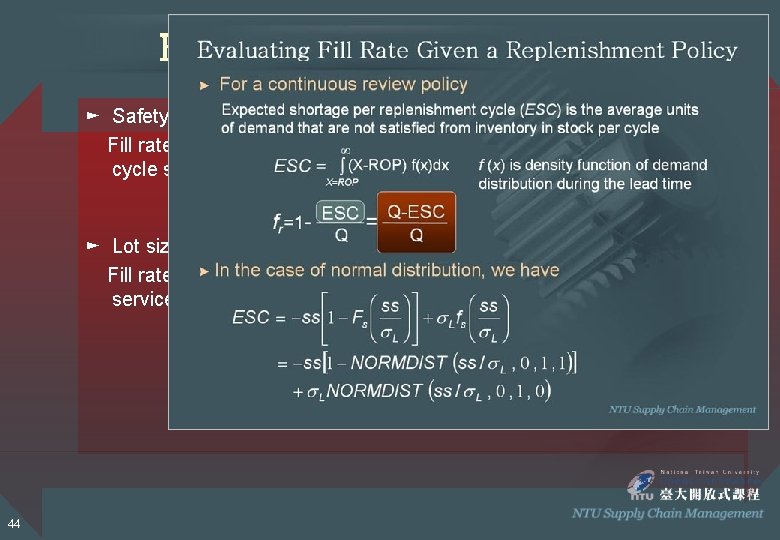
Evaluating Fill Rate Given a Replenishment Policy ► For a continuous review policy Expected shortage per replenishment cycle (ESC) is the average units of demand that are not satisfied from inventory in stock per cycle ¥ ESC = ò (X-ROP) f(x)dx X=ROP f (x) is density function of demand distribution during the lead time fr=1 - ESC = Q-ESC Q Q ► In the case of normal distribution, we have 29

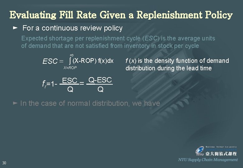
Evaluating Fill Rate Given a Replenishment Policy ► For a continuous review policy Expected shortage per replenishment cycle (ESC) is the average units of demand that are not satisfied from inventory in stock per cycle ¥ ESC = ò (X-ROP) f(x)dx X=ROP f (x) is the density function of demand distribution during the lead time fr=1 - ESC = Q-ESC Q Q ► In the case of normal distribution, we have 30

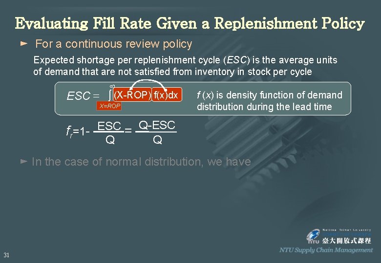
Evaluating Fill Rate Given a Replenishment Policy ► For a continuous review policy Expected shortage per replenishment cycle (ESC) is the average units of demand that are not satisfied from inventory in stock per cycle ¥ ESC = ò (X-ROP) f(x)dx X=ROP f (x) is density function of demand distribution during the lead time fr=1 - ESC = Q-ESC Q Q ► In the case of normal distribution, we have 31

Evaluating Fill Rate Given a Replenishment Policy ► For a continuous review policy Expected shortage per replenishment cycle (ESC) is the average units of demand that are not satisfied from inventory in stock per cycle ¥ ESC = ò (X-ROP) f(x)dx X=ROP f (x) is density function of demand distribution during the lead time fr=1 - ESC = Q-ESC Q Q ► In the case of normal distribution, we have 32

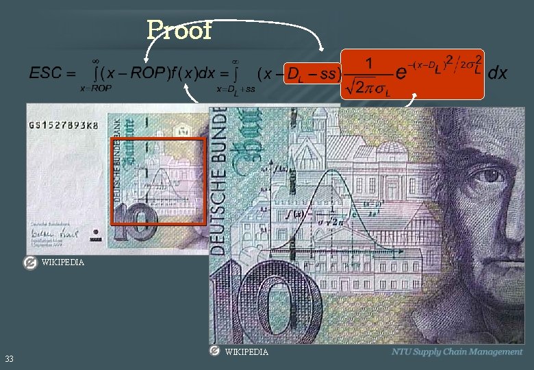
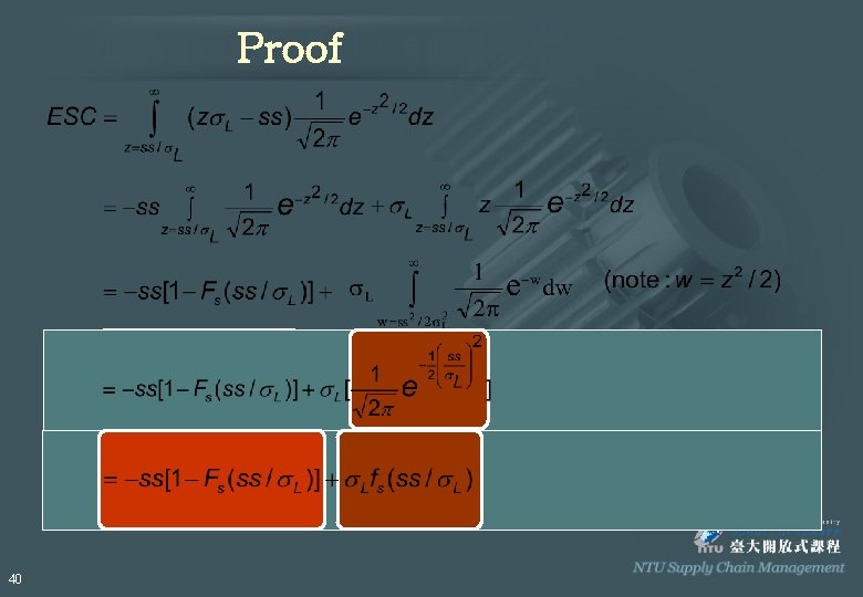
Proof WIKIPEDIA 33 WIKIPEDIA

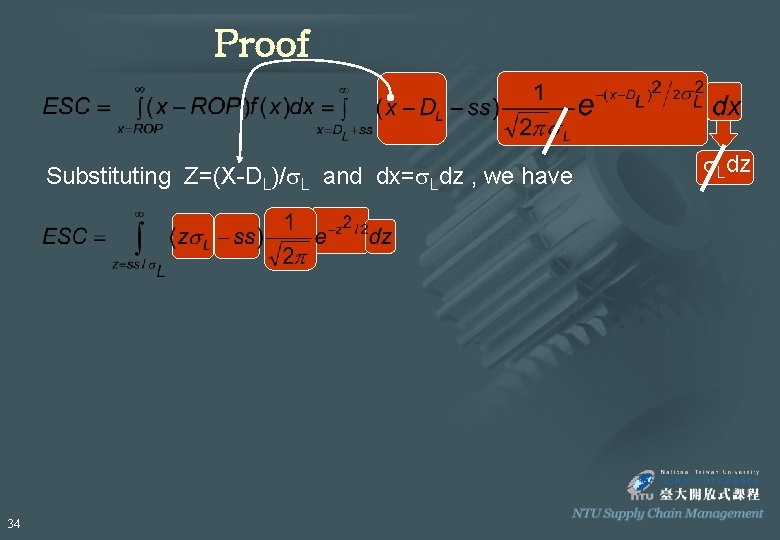
Proof Substituting Z=(X-DL)/s. L and dx=s. Ldz , we have 34 s. Ldz

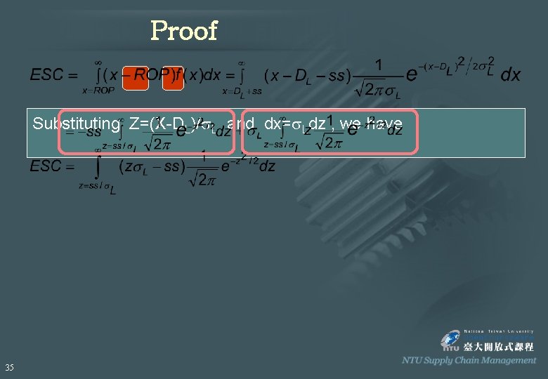
Proof Substituting Z=(X-DL)/s. L and dx=s. Ldz , we have 35

Proof 36

Proof 37

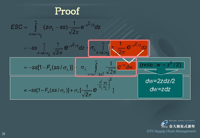
Proof dw=2 zdz/2 dw=zdz 38

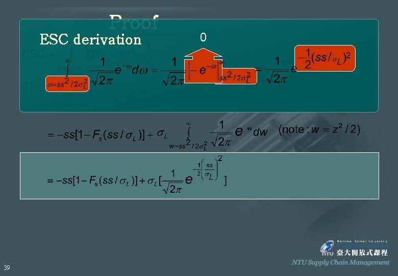
Proof ESC derivation 39 0

Proof 40

Evaluating Fill Rate Given a Replenishment Policy ► For a continuous review policy Expected shortage per replenishment cycle (ESC) is the average units of demand that are not satisfied from inventory in stock per cycle ¥ ESC = ò (X-ROP) f(x)dx X=ROP f (x) is density function of demand distribution during the lead time fr=1 - ESC = Q-ESC Q Q ► In the case of normal distribution, we have 41

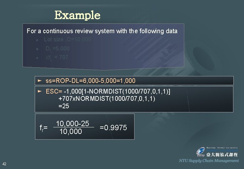
Example For a continuous review system with the following data u u u Lot size , Q=10, 000 DL=5, 000 s. L = 707 ► ss=ROP-DL=6, 000 -5, 000=1, 000 ► ESC= -1, 000[1 -NORMDIST(1000/707, 0, 1, 1)] +707 x. NORMDIST(1000/707, 0, 1, 1) =25 f r= 42 10, 000 -25 10, 000 =0. 9975

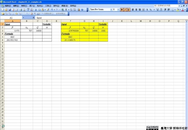
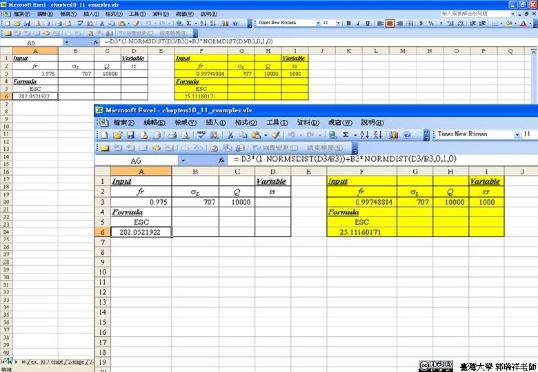
Excel-Demo For a continuous review system with the following data 5 Lot size , Q=10, 000 5 5 DL=5, 000 s. L = 707 > ss=ROP-DL=6, 000 -5, 000=1, 000 > ESC= -1, 000[1 -NORMDIST(1000/707, 0, 1, 1)] +707 x. NORMDIST(1000/707, 0, 1, 1) =25 f r= 43 10, 000 -25 10, 000 =0. 9975 臺灣大學 郭瑞祥老師

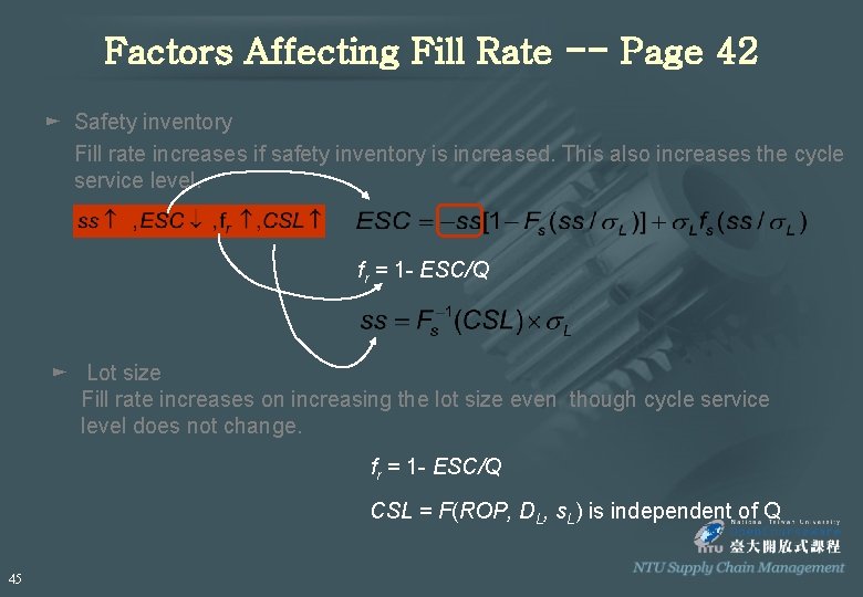
Factors Affecting Fill Rate ► Safety inventory Fill rate increases if safety inventory is increased. This also increases the cycle service level. ► Lot size Fill rate increases with the increase of the lot size even though cycle service level does not change. 44

Factors Affecting Fill Rate -- Page 42 ► Safety inventory Fill rate increases if safety inventory is increased. This also increases the cycle service level. fr = 1 - ESC/Q ► Lot size Fill rate increases on increasing the lot size even though cycle service level does not change. fr = 1 - ESC/Q CSL = F(ROP, DL, s. L) is independent of Q 45

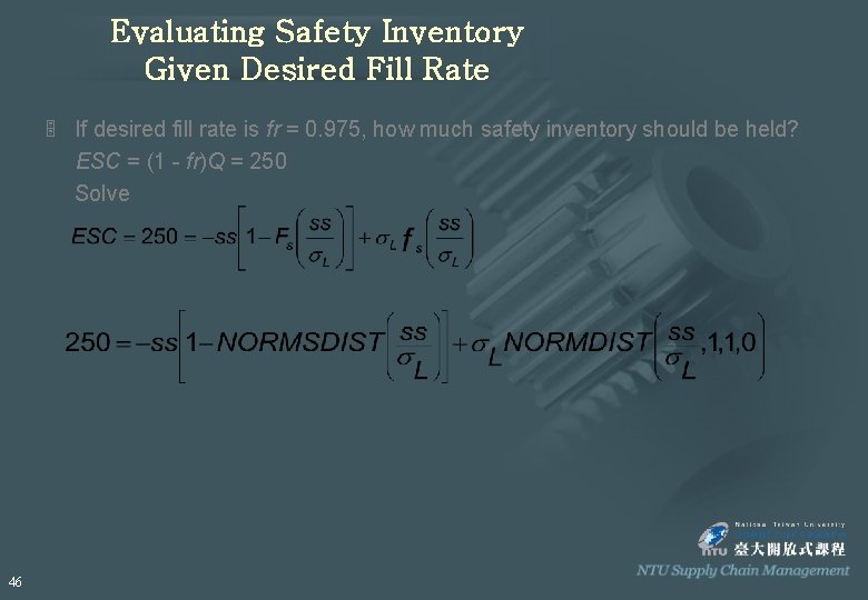
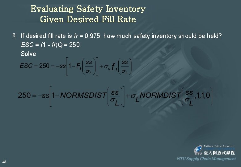
Evaluating Safety Inventory Given Desired Fill Rate 5 If desired fill rate is fr = 0. 975, how much safety inventory should be held? ESC = (1 - fr)Q = 250 Solve 46

Evaluating Safety Inventory Given Desired Fill Rate 5 If desired fill rate is fr = 0. 975, how much safety inventory should be held? ESC = (1 - fr)Q = 250 Solve 48

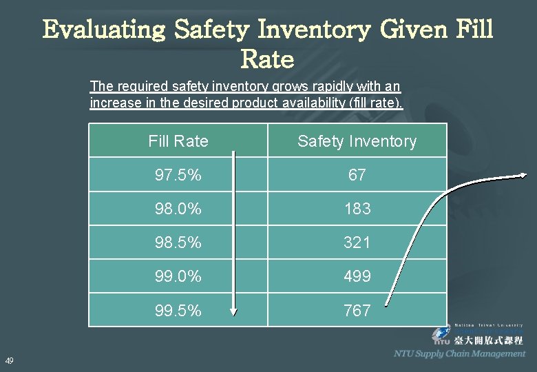
Evaluating Safety Inventory Given Fill Rate The required safety inventory grows rapidly with an increase in the desired product availability (fill rate). 49 Fill Rate Safety Inventory 97. 5% 67 98. 0% 183 98. 5% 321 99. 0% 499 99. 5% 767

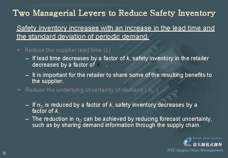
Two Managerial Levers to Reduce Safety Inventory Safety inventory increases with an increase in the lead time and the standard deviation of periodic demand. ► Reduce the supplier lead time (L) – If lead time decreases by a factor of k, safety inventory in the retailer decreases by a factor of. – It is important for the retailer to share some of the resulting benefits to the supplier. ► Reduce the underlying uncertainty of demand ( s. D ) – If s. D is reduced by a factor of k, safety inventory decreases by a factor of k. – The reduction in s. D can be achieved by reducing forecast uncertainty, such as by sharing demand information through the supply chain. 50

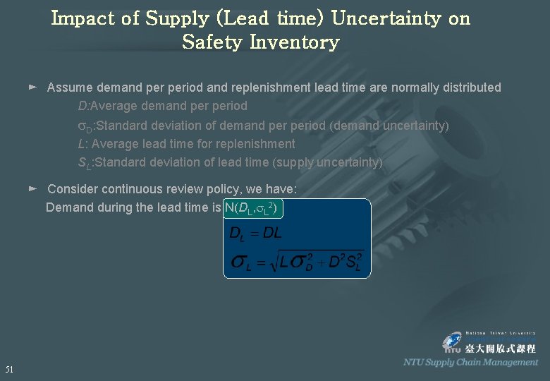
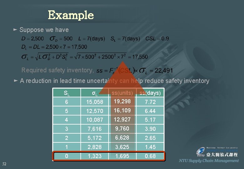
Impact of Supply (Lead time) Uncertainty on Safety Inventory ► Assume demand period and replenishment lead time are normally distributed D: Average demand period s. D: Standard deviation of demand period (demand uncertainty) L: Average lead time for replenishment SL: Standard deviation of lead time (supply uncertainty) ► Consider continuous review policy, we have: Demand during the lead time is N(DL, s. L 2) 51

Example ► Suppose we have Required safety inventory, ► A reduction in lead time uncertainty can help reduce safety inventory 52 SL σL ss(units) ss(days) 6 15, 058 19, 298 7. 72 5 12, 570 16, 109 6. 44 4 10, 087 12, 927 5. 17 3 7, 616 9, 760 3. 90 2 5, 172 6, 628 2. 65 1 2, 828 3, 625 1. 45 0 1, 323 1, 695 0. 68

版權聲明 頁碼 53 作品 授權條件 作者/來源 5 本作品轉載自Cool. CLIPS網站 (http: //dir. coolclips. com/Popular/World_of_Industry/Food/Shopping_cart_full_of_gr oceries_vc 012266. html )，瀏覽日期 2011/12/28。依據著作權法第 46、52、65條 合理使用。 6 本作品轉載自 WIKIPEDIA(http: //en. wikipedia. org/wiki/File: Palm-m 505. jpg)，瀏 覽日期 2012/2/21。 6 本作品轉載自Microsoft Office 2007多媒體藝廊，依據Microsoft 服務合約及著 作權法第 46、52、65條合理使用。 19 臺灣大學 郭瑞祥老師 22 臺灣大學 郭瑞祥老師