CS 4803 7643 Deep Learning Topics Variational AutoEncoders

CS 4803 / 7643: Deep Learning Topics: – Variational Auto-Encoders (VAEs) – AEs, Variational Inference Dhruv Batra Georgia Tech

Administrativia • HW 4 Reminder – Due: 11/07, 11: 55 pm – Reinforcement Learning – Last HW. Focus on project after that. • Final project – No poster session – PDF Report submission • Details out soon (C) Dhruv Batra 2

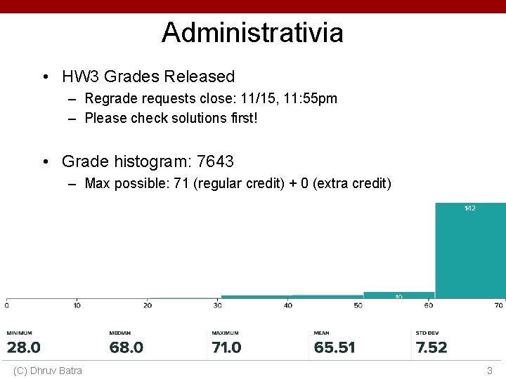
Administrativia • HW 3 Grades Released – Regrade requests close: 11/15, 11: 55 pm – Please check solutions first! • Grade histogram: 7643 – Max possible: 71 (regular credit) + 0 (extra credit) (C) Dhruv Batra 3

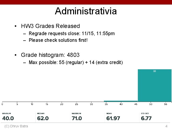
Administrativia • HW 3 Grades Released – Regrade requests close: 11/15, 11: 55 pm – Please check solutions first! • Grade histogram: 4803 – Max possible: 55 (regular) + 14 (extra credit) (C) Dhruv Batra 4

Recap from last time 2 lectures ago (C) Dhruv Batra 5

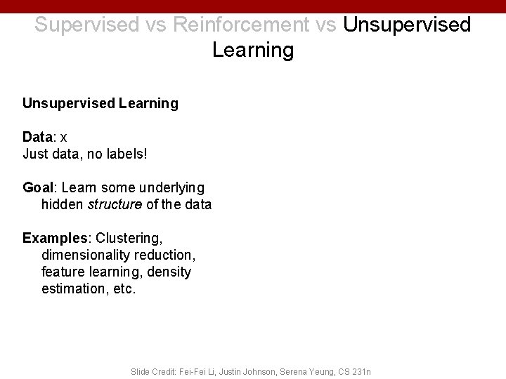
Supervised vs Reinforcement vs Unsupervised Learning Slide Credit: Fei-Fei Li, Justin Johnson, Serena Yeung, CS 231 n

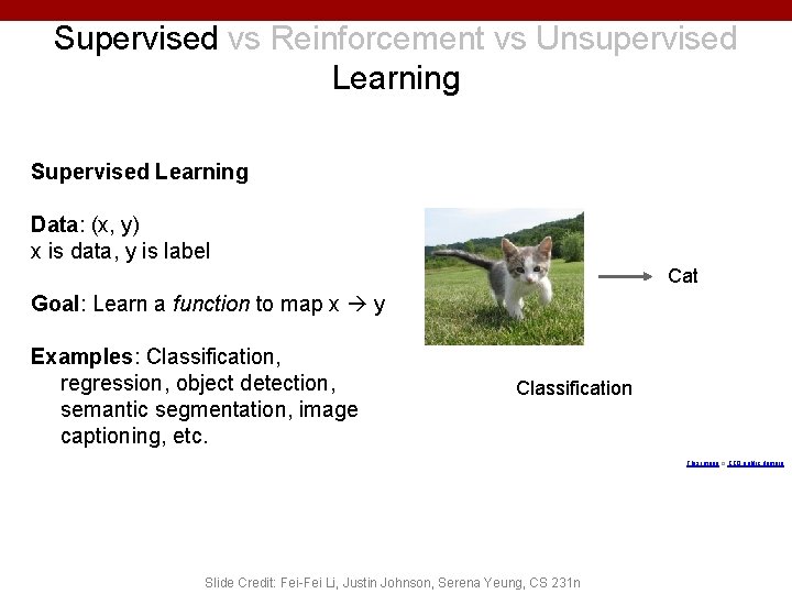
Supervised vs Reinforcement vs Unsupervised Learning Supervised Learning Data: (x, y) x is data, y is label Cat Goal: Learn a function to map x y Examples: Classification, regression, object detection, semantic segmentation, image captioning, etc. Classification This image is CC 0 public domain Slide Credit: Fei-Fei Li, Justin Johnson, Serena Yeung, CS 231 n

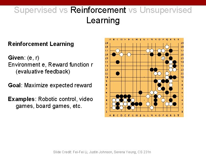
Supervised vs Reinforcement vs Unsupervised Learning Reinforcement Learning Given: (e, r) Environment e, Reward function r (evaluative feedback) Goal: Maximize expected reward Examples: Robotic control, video games, board games, etc. Slide Credit: Fei-Fei Li, Justin Johnson, Serena Yeung, CS 231 n

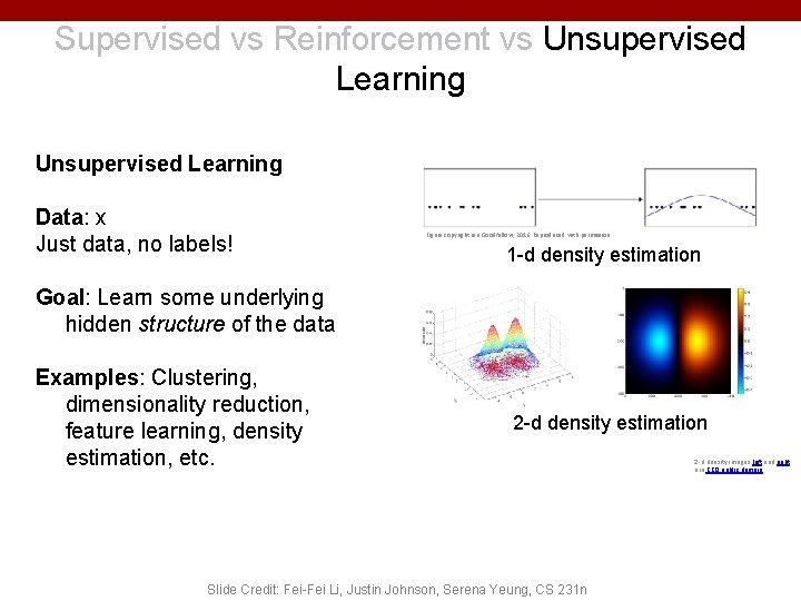
Supervised vs Reinforcement vs Unsupervised Learning Data: x Just data, no labels! Goal: Learn some underlying hidden structure of the data Examples: Clustering, dimensionality reduction, feature learning, density estimation, etc. Slide Credit: Fei-Fei Li, Justin Johnson, Serena Yeung, CS 231 n

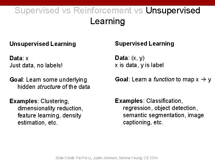
Supervised vs Reinforcement vs Unsupervised Learning Supervised Learning Data: x Just data, no labels! Data: (x, y) x is data, y is label Goal: Learn some underlying hidden structure of the data Goal: Learn a function to map x y Examples: Clustering, dimensionality reduction, feature learning, density estimation, etc. Examples: Classification, regression, object detection, semantic segmentation, image captioning, etc. Slide Credit: Fei-Fei Li, Justin Johnson, Serena Yeung, CS 231 n

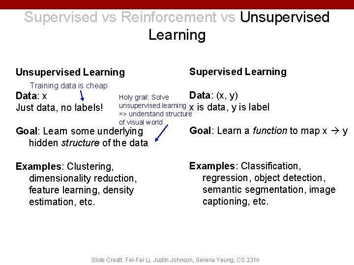
Supervised vs Reinforcement vs Unsupervised Learning Training data is cheap Data: x Just data, no labels! Supervised Learning Data: (x, y) Holy grail: Solve unsupervised learning x is data, y is label => understand structure of visual world Goal: Learn some underlying hidden structure of the data Goal: Learn a function to map x y Examples: Clustering, dimensionality reduction, feature learning, density estimation, etc. Examples: Classification, regression, object detection, semantic segmentation, image captioning, etc. Slide Credit: Fei-Fei Li, Justin Johnson, Serena Yeung, CS 231 n

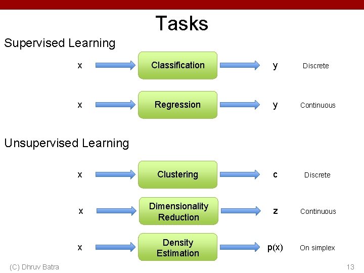
Tasks Supervised Learning x Classification y Discrete x Regression y Continuous x Clustering c Discrete x Dimensionality Reduction z Continuous x Density Estimation p(x) On simplex Unsupervised Learning (C) Dhruv Batra 13

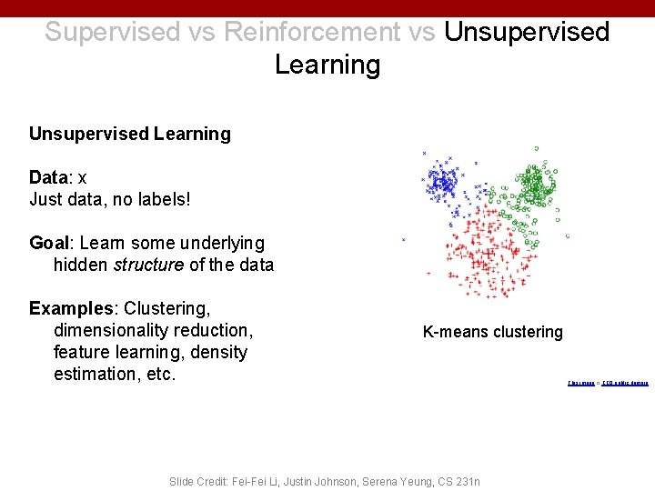
Supervised vs Reinforcement vs Unsupervised Learning Data: x Just data, no labels! Goal: Learn some underlying hidden structure of the data Examples: Clustering, dimensionality reduction, feature learning, density estimation, etc. K-means clustering Slide Credit: Fei-Fei Li, Justin Johnson, Serena Yeung, CS 231 n This image is CC 0 public domain

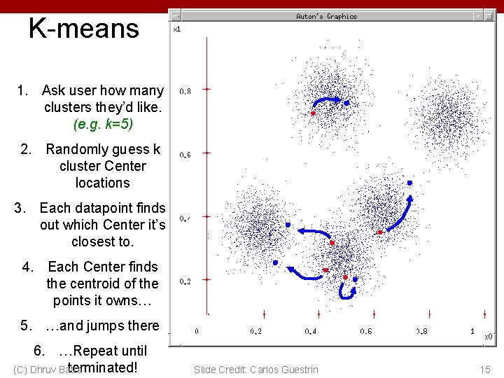
K-means 1. Ask user how many clusters they’d like. (e. g. k=5) 2. Randomly guess k cluster Center locations 3. Each datapoint finds out which Center it’s closest to. 4. Each Center finds the centroid of the points it owns… 5. …and jumps there 6. …Repeat until terminated! (C) Dhruv Batra Slide Credit: Carlos Guestrin 15

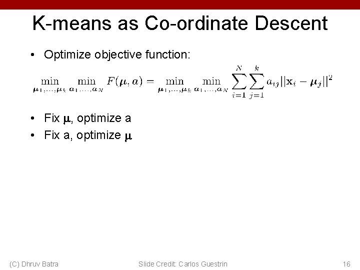
K-means as Co-ordinate Descent • Optimize objective function: • Fix , optimize a • Fix a, optimize (C) Dhruv Batra Slide Credit: Carlos Guestrin 16

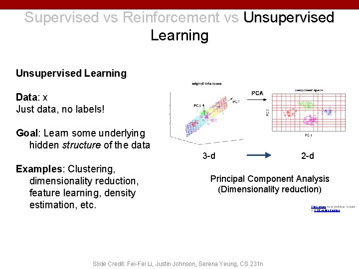
Supervised vs Reinforcement vs Unsupervised Learning Data: x Just data, no labels! Goal: Learn some underlying hidden structure of the data 3 -d Examples: Clustering, dimensionality reduction, feature learning, density estimation, etc. 2 -d Principal Component Analysis (Dimensionality reduction) Slide Credit: Fei-Fei Li, Justin Johnson, Serena Yeung, CS 231 n This image from Matthias Scholz is CC 0 public domain

Supervised vs Reinforcement vs Unsupervised Learning Data: x Just data, no labels! Figure copyright Ian Goodfellow, 2016. Reproduced with permission. 1 -d density estimation Goal: Learn some underlying hidden structure of the data Examples: Clustering, dimensionality reduction, feature learning, density estimation, etc. 2 -d density estimation Slide Credit: Fei-Fei Li, Justin Johnson, Serena Yeung, CS 231 n 2 -d density images left and right are CC 0 public domain

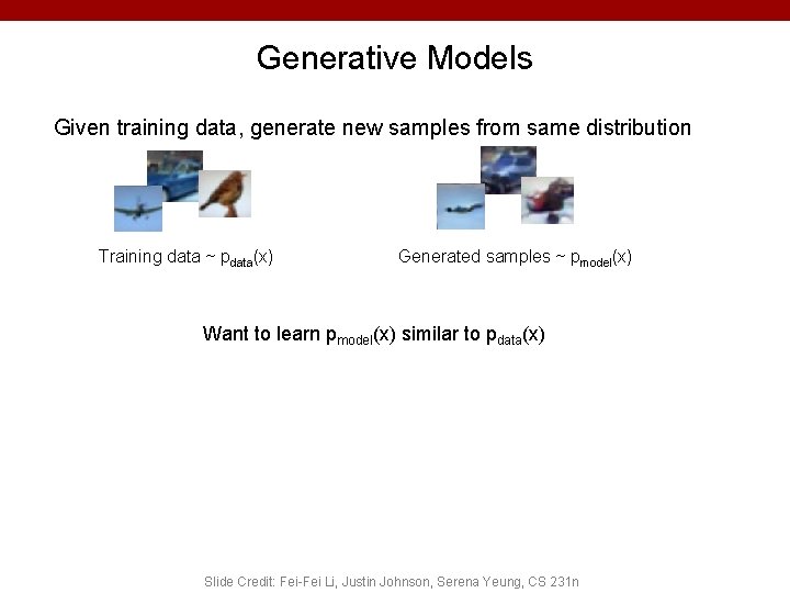
Generative Models Given training data, generate new samples from same distribution Training data ~ pdata(x) Generated samples ~ pmodel(x) Want to learn pmodel(x) similar to pdata(x) Slide Credit: Fei-Fei Li, Justin Johnson, Serena Yeung, CS 231 n

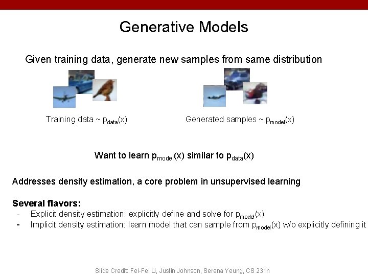
Generative Models Given training data, generate new samples from same distribution Training data ~ pdata(x) Generated samples ~ pmodel(x) Want to learn pmodel(x) similar to pdata(x) Addresses density estimation, a core problem in unsupervised learning Several flavors: - - Explicit density estimation: explicitly define and solve for pmodel(x) Implicit density estimation: learn model that can sample from pmodel(x) w/o explicitly defining it Slide Credit: Fei-Fei Li, Justin Johnson, Serena Yeung, CS 231 n

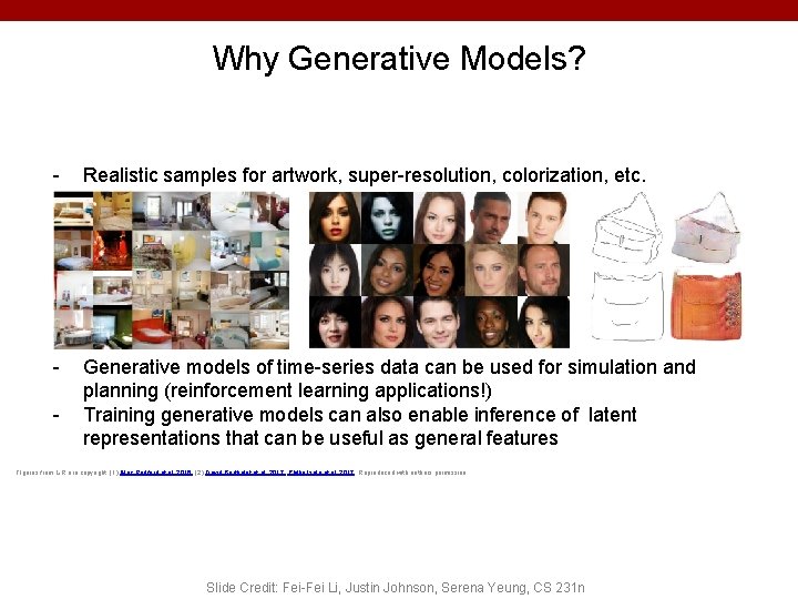
Why Generative Models? - Realistic samples for artwork, super-resolution, colorization, etc. - Generative models of time-series data can be used for simulation and planning (reinforcement learning applications!) Training generative models can also enable inference of latent representations that can be useful as general features - FIgures from L-R are copyright: (1) Alec Radford et al. 2016; (2) David Berthelot et al. 2017; Phillip Isola et al. 2017. Reproduced with authors permission. Slide Credit: Fei-Fei Li, Justin Johnson, Serena Yeung, CS 231 n

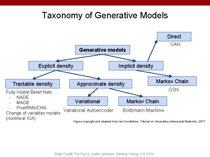
Taxonomy of Generative Models Direct GAN Generative models Explicit density Tractable density Implicit density Markov Chain Approximate density Fully Visible Belief Nets - NADE Variational - MADE - Pixel. RNN/CNN Variational Autoencoder Change of variables models (nonlinear ICA) GSN Markov Chain Boltzmann Machine Figure copyright and adapted from Ian Goodfellow, Tutorial on Generative Adversarial Networks, 2017. Slide Credit: Fei-Fei Li, Justin Johnson, Serena Yeung, CS 231 n

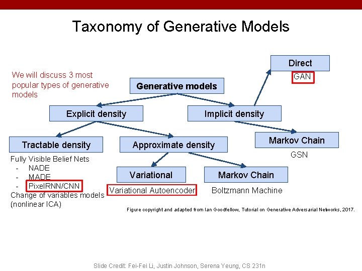
Taxonomy of Generative Models Direct We will discuss 3 most popular types of generative models GAN Generative models Explicit density Tractable density Implicit density Markov Chain Approximate density Fully Visible Belief Nets - NADE Variational - MADE - Pixel. RNN/CNN Variational Autoencoder Change of variables models (nonlinear ICA) GSN Markov Chain Boltzmann Machine Figure copyright and adapted from Ian Goodfellow, Tutorial on Generative Adversarial Networks, 2017. Slide Credit: Fei-Fei Li, Justin Johnson, Serena Yeung, CS 231 n

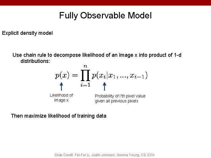
Fully Observable Model Explicit density model Use chain rule to decompose likelihood of an image x into product of 1 -d distributions: Likelihood of image x Probability of i’th pixel value given all previous pixels Then maximize likelihood of training data Slide Credit: Fei-Fei Li, Justin Johnson, Serena Yeung, CS 231 n

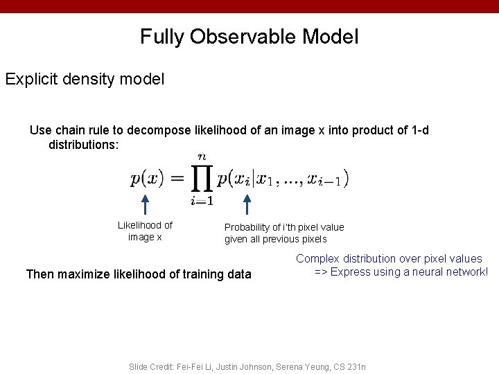
Fully Observable Model Explicit density model Use chain rule to decompose likelihood of an image x into product of 1 -d distributions: Likelihood of image x Probability of i’th pixel value given all previous pixels Then maximize likelihood of training data Complex distribution over pixel values => Express using a neural network! Slide Credit: Fei-Fei Li, Justin Johnson, Serena Yeung, CS 231 n

Plan for Today • Goal: Variational Autoencoders • Latent variable probabilistic models – Example GMMs • Autoencodeders • Variational Inference (C) Dhruv Batra 26

Variational Autoencoders (VAE)

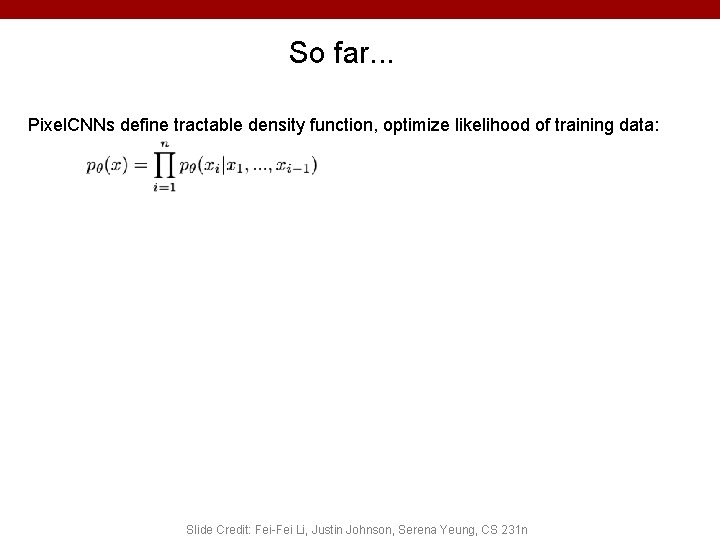
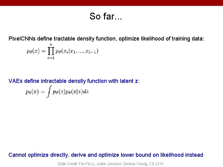
So far. . . Pixel. CNNs define tractable density function, optimize likelihood of training data: Slide Credit: Fei-Fei Li, Justin Johnson, Serena Yeung, CS 231 n

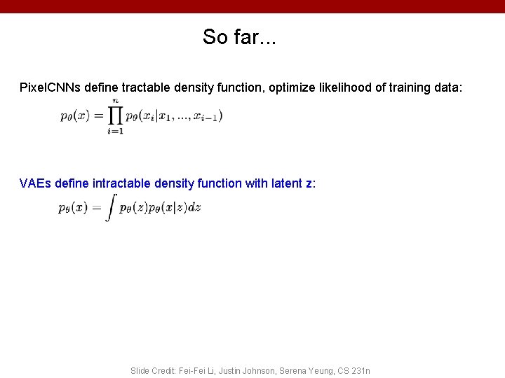
So far. . . Pixel. CNNs define tractable density function, optimize likelihood of training data: VAEs define intractable density function with latent z: Slide Credit: Fei-Fei Li, Justin Johnson, Serena Yeung, CS 231 n

So far. . . Pixel. CNNs define tractable density function, optimize likelihood of training data: VAEs define intractable density function with latent z: Cannot optimize directly, derive and optimize lower bound on likelihood instead Slide Credit: Fei-Fei Li, Justin Johnson, Serena Yeung, CS 231 n

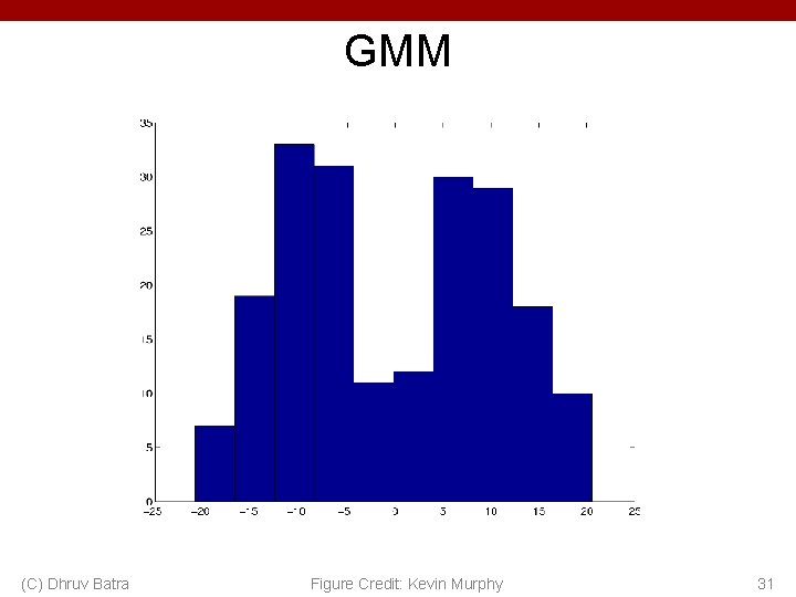
GMM (C) Dhruv Batra Figure Credit: Kevin Murphy 31

Gaussian Mixture Model (C) Dhruv Batra 32

Gaussian Mixture Model (C) Dhruv Batra 33

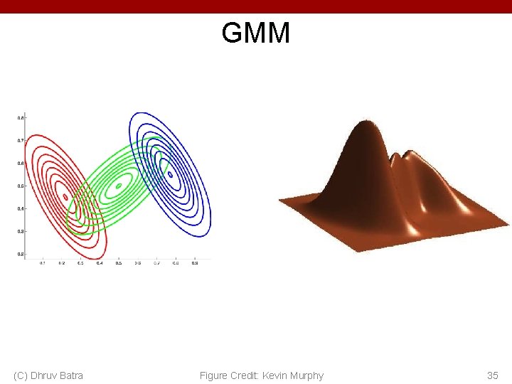
GMM (C) Dhruv Batra Figure Credit: Kevin Murphy 35

K-means vs GMM • K-Means – http: //stanford. edu/class/ee 103/visualizations/kmean s. html • GMM – https: //lukapopijac. github. io/gaussian-mixture-model/ (C) Dhruv Batra 36

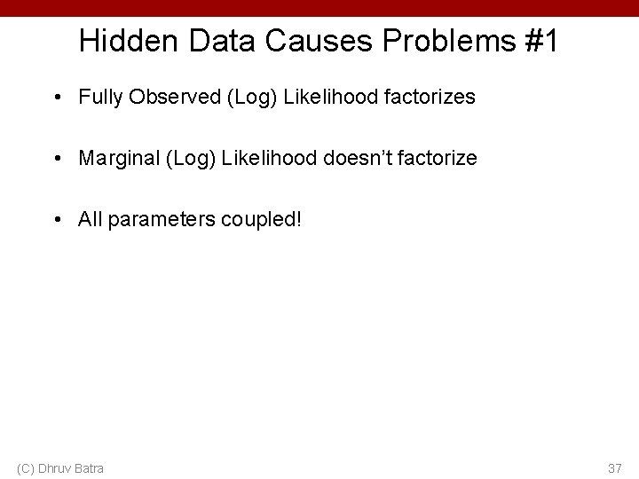
Hidden Data Causes Problems #1 • Fully Observed (Log) Likelihood factorizes • Marginal (Log) Likelihood doesn’t factorize • All parameters coupled! (C) Dhruv Batra 37

(C) Dhruv Batra 38

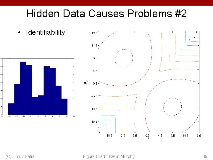
Hidden Data Causes Problems #2 • Identifiability (C) Dhruv Batra Figure Credit: Kevin Murphy 39

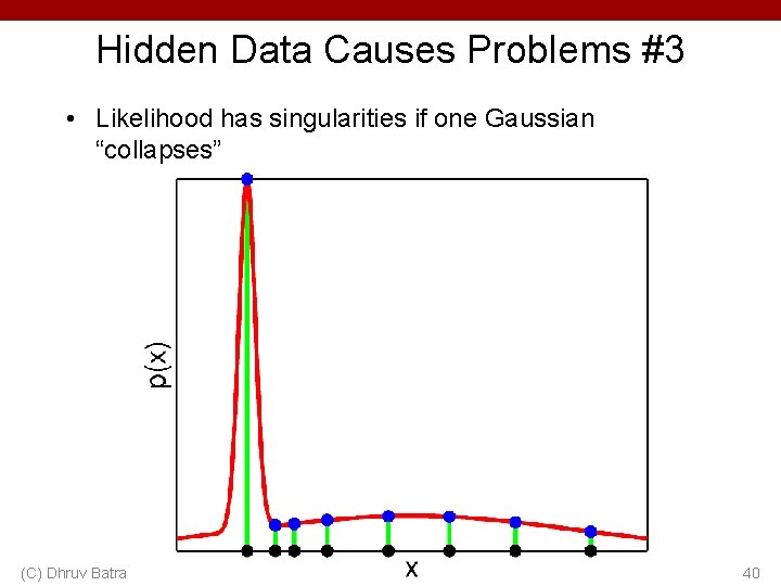
Hidden Data Causes Problems #3 • Likelihood has singularities if one Gaussian “collapses” (C) Dhruv Batra 40

(C) Dhruv Batra 41

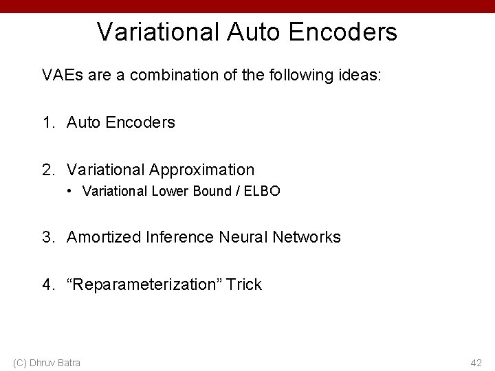
Variational Auto Encoders VAEs are a combination of the following ideas: 1. Auto Encoders 2. Variational Approximation • Variational Lower Bound / ELBO 3. Amortized Inference Neural Networks 4. “Reparameterization” Trick (C) Dhruv Batra 42

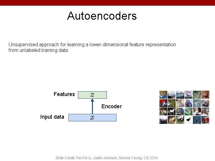
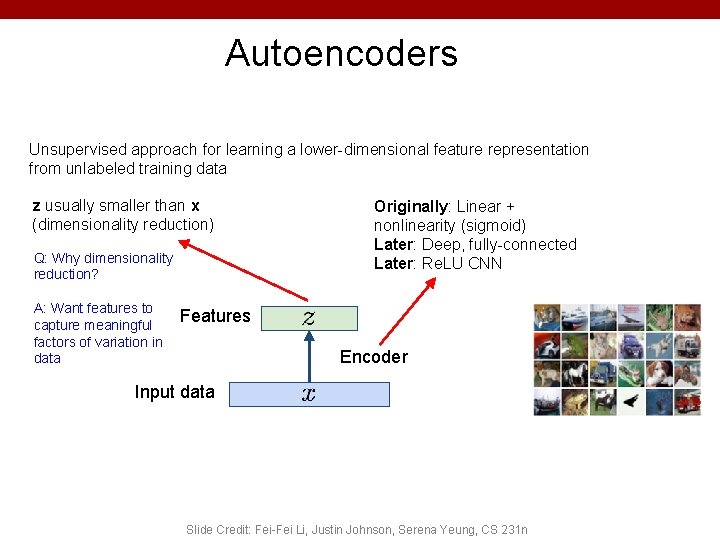
Autoencoders Unsupervised approach for learning a lower-dimensional feature representation from unlabeled training data Features Encoder Input data Slide Credit: Fei-Fei Li, Justin Johnson, Serena Yeung, CS 231 n

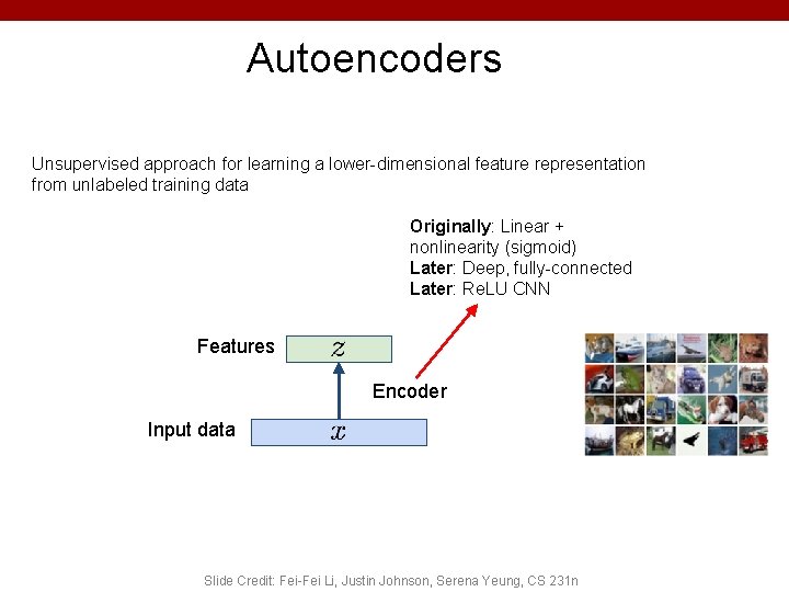
Autoencoders Unsupervised approach for learning a lower-dimensional feature representation from unlabeled training data Originally: Linear + nonlinearity (sigmoid) Later: Deep, fully-connected Later: Re. LU CNN Features Encoder Input data Slide Credit: Fei-Fei Li, Justin Johnson, Serena Yeung, CS 231 n

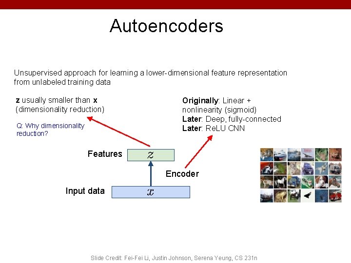
Autoencoders Unsupervised approach for learning a lower-dimensional feature representation from unlabeled training data z usually smaller than x (dimensionality reduction) Q: Why dimensionality reduction? Originally: Linear + nonlinearity (sigmoid) Later: Deep, fully-connected Later: Re. LU CNN Features Encoder Input data Slide Credit: Fei-Fei Li, Justin Johnson, Serena Yeung, CS 231 n

Autoencoders Unsupervised approach for learning a lower-dimensional feature representation from unlabeled training data z usually smaller than x (dimensionality reduction) Q: Why dimensionality reduction? A: Want features to capture meaningful factors of variation in data Originally: Linear + nonlinearity (sigmoid) Later: Deep, fully-connected Later: Re. LU CNN Features Encoder Input data Slide Credit: Fei-Fei Li, Justin Johnson, Serena Yeung, CS 231 n

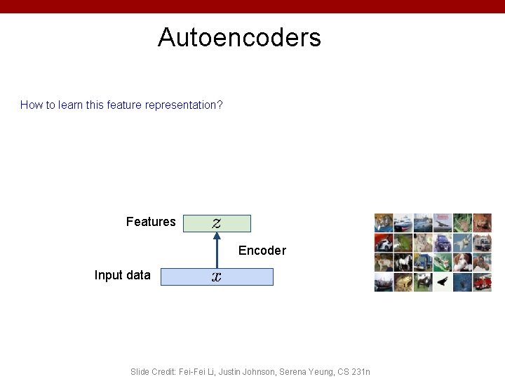
Autoencoders How to learn this feature representation? Features Encoder Input data Slide Credit: Fei-Fei Li, Justin Johnson, Serena Yeung, CS 231 n

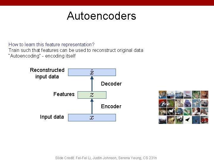
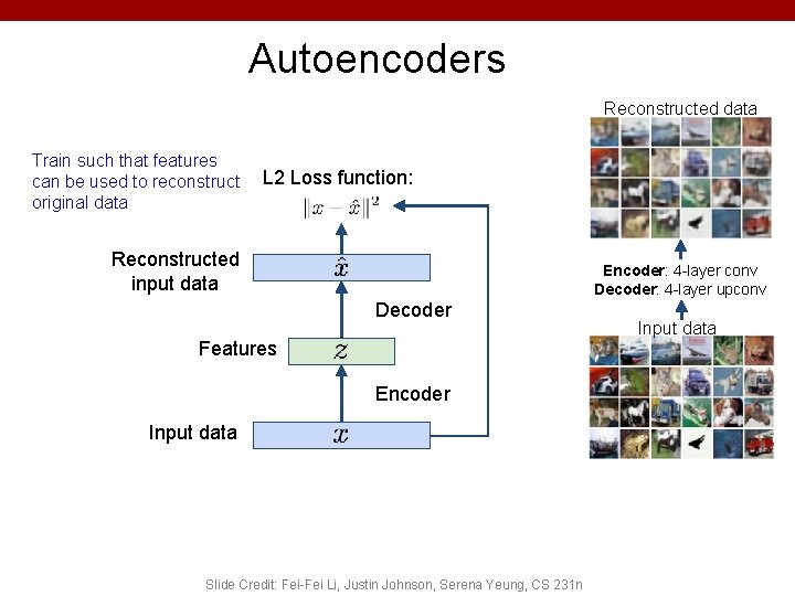
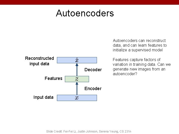
Autoencoders How to learn this feature representation? Train such that features can be used to reconstruct original data “Autoencoding” - encoding itself Reconstructed input data Decoder Features Encoder Input data Slide Credit: Fei-Fei Li, Justin Johnson, Serena Yeung, CS 231 n

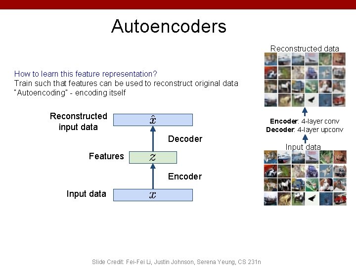
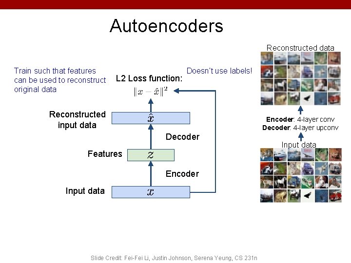
Autoencoders Reconstructed data How to learn this feature representation? Train such that features can be used to reconstruct original data “Autoencoding” - encoding itself Reconstructed input data Encoder: 4 -layer conv Decoder: 4 -layer upconv Decoder Features Encoder Input data Slide Credit: Fei-Fei Li, Justin Johnson, Serena Yeung, CS 231 n Input data

Autoencoders Reconstructed data Train such that features can be used to reconstruct original data L 2 Loss function: Reconstructed input data Encoder: 4 -layer conv Decoder: 4 -layer upconv Decoder Features Encoder Input data Slide Credit: Fei-Fei Li, Justin Johnson, Serena Yeung, CS 231 n Input data

Autoencoders Reconstructed data Train such that features can be used to reconstruct original data L 2 Loss function: Doesn’t use labels! Reconstructed input data Encoder: 4 -layer conv Decoder: 4 -layer upconv Decoder Features Encoder Input data Slide Credit: Fei-Fei Li, Justin Johnson, Serena Yeung, CS 231 n Input data

Autoencoders • Demo – https: //cs. stanford. edu/people/karpathy/convnetjs/demo/auto encoder. html 53

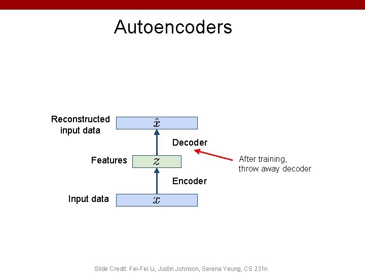
Autoencoders Reconstructed input data Decoder After training, throw away decoder Features Encoder Input data Slide Credit: Fei-Fei Li, Justin Johnson, Serena Yeung, CS 231 n

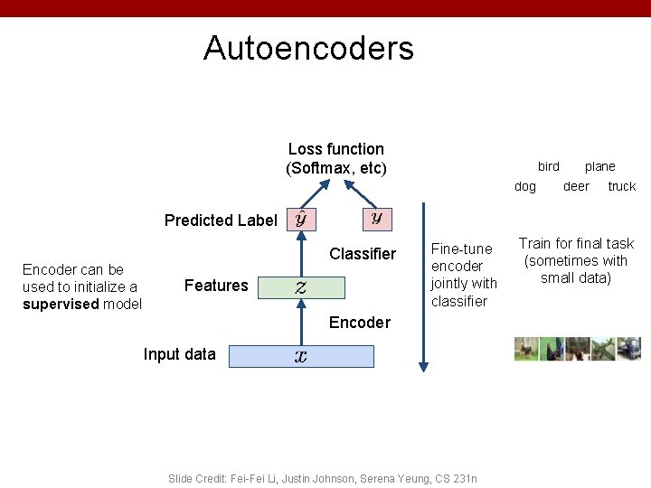
Autoencoders Loss function (Softmax, etc) bird dog plane deer truck Predicted Label Encoder can be used to initialize a supervised model Classifier Features Fine-tune encoder jointly with classifier Encoder Input data Slide Credit: Fei-Fei Li, Justin Johnson, Serena Yeung, CS 231 n Train for final task (sometimes with small data)

Autoencoders can reconstruct data, and can learn features to initialize a supervised model Reconstructed input data Decoder Features capture factors of variation in training data. Can we generate new images from an autoencoder? Encoder Input data Slide Credit: Fei-Fei Li, Justin Johnson, Serena Yeung, CS 231 n

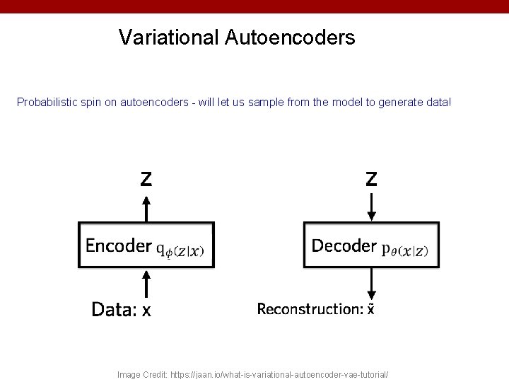
Variational Autoencoders Probabilistic spin on autoencoders - will let us sample from the model to generate data! Image Credit: https: //jaan. io/what-is-variational-autoencoder-vae-tutorial/

Variational Auto Encoders VAEs are a combination of the following ideas: 1. Auto Encoders 2. Variational Approximation • Variational Lower Bound / ELBO 3. Amortized Inference Neural Networks 4. “Reparameterization” Trick (C) Dhruv Batra 58

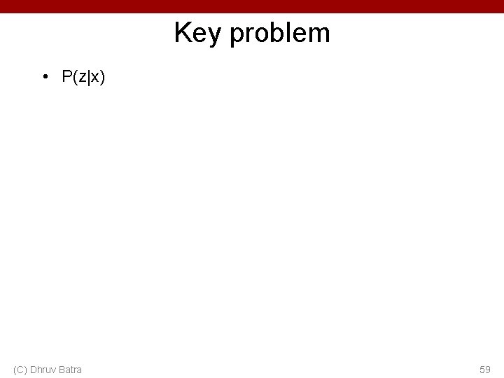
Key problem • P(z|x) (C) Dhruv Batra 59

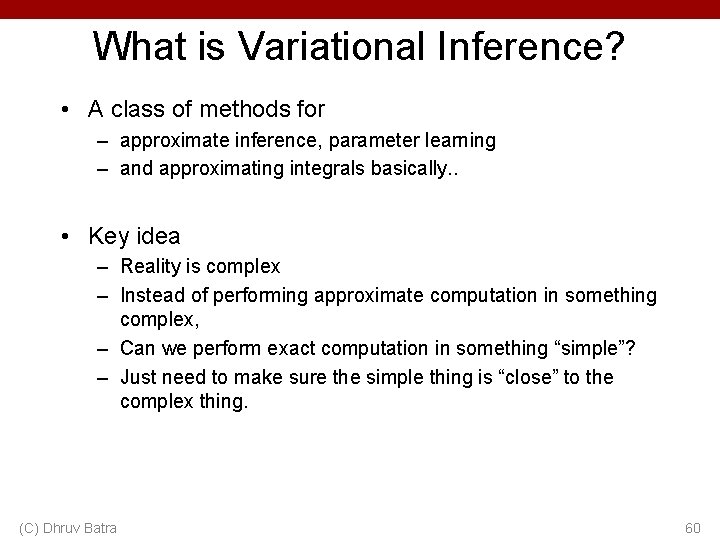
What is Variational Inference? • A class of methods for – approximate inference, parameter learning – and approximating integrals basically. . • Key idea – Reality is complex – Instead of performing approximate computation in something complex, – Can we perform exact computation in something “simple”? – Just need to make sure the simple thing is “close” to the complex thing. (C) Dhruv Batra 60

Intuition (C) Dhruv Batra 61

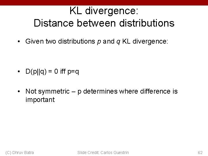
KL divergence: Distance between distributions • Given two distributions p and q KL divergence: • D(p||q) = 0 iff p=q • Not symmetric – p determines where difference is important (C) Dhruv Batra Slide Credit: Carlos Guestrin 62

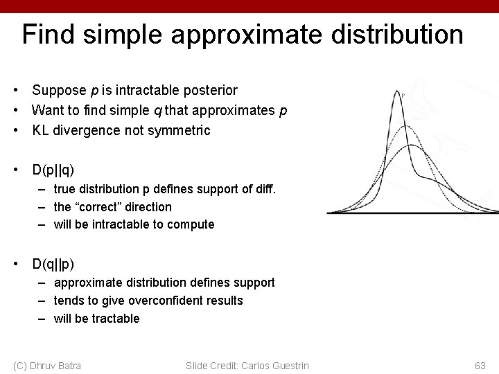
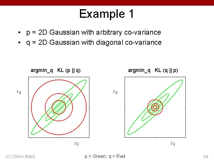
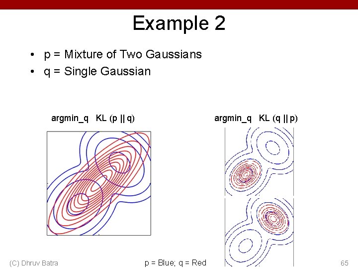
Find simple approximate distribution • Suppose p is intractable posterior • Want to find simple q that approximates p • KL divergence not symmetric • D(p||q) – true distribution p defines support of diff. – the “correct” direction – will be intractable to compute • D(q||p) – approximate distribution defines support – tends to give overconfident results – will be tractable (C) Dhruv Batra Slide Credit: Carlos Guestrin 63

Example 1 • p = 2 D Gaussian with arbitrary co-variance • q = 2 D Gaussian with diagonal co-variance argmin_q KL (p || q) (C) Dhruv Batra argmin_q KL (q || p) p = Green; q = Red 64

Example 2 • p = Mixture of Two Gaussians • q = Single Gaussian argmin_q KL (p || q) (C) Dhruv Batra argmin_q KL (q || p) p = Blue; q = Red 65