A Fem Variational approach to the droplet spreading

A Fem. Variational approach to the droplet spreading over dry surfaces S. Manservisi Nuclear Engineering Lab. of Montecuccolino University of Bologna, Italy Department of mathematics Texas Tech University, USA

Simulations of droplets impacting orthogonally over dry surfaces at Low Reynolds Numbers OUTLINE OF THE PRESENTATION - Introduction to the impact problem - Front tracking method - Variational formulation of the contact pro - Numerical experiments

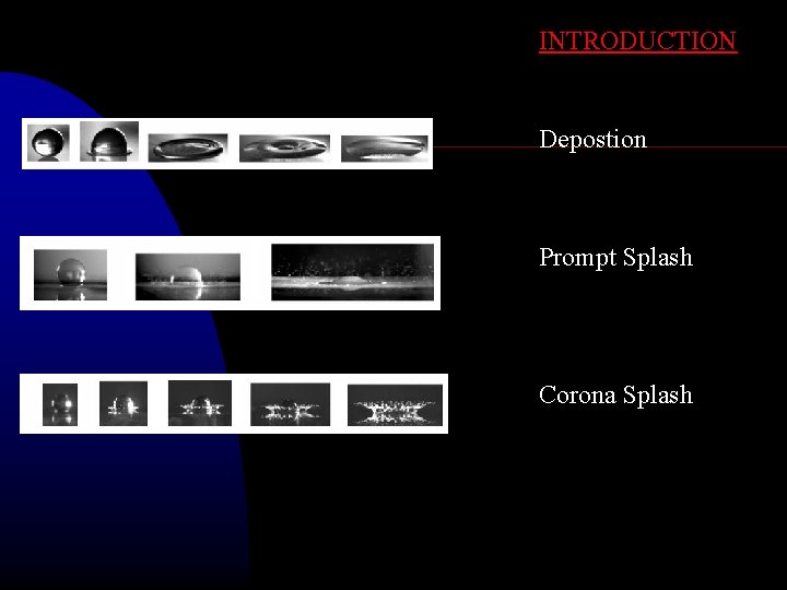
INTRODUCTION Depostion Prompt Splashd Corona Splashd

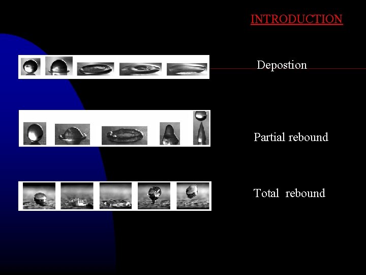
INTRODUCTION Depostion Partial reboundd Total reboundd

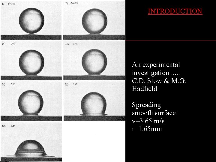
INTRODUCTION An experimental investigation. . . C. D. Stow & M. G. Hadfield Spreading smooth surface v=3. 65 m/s r=1. 65 mm

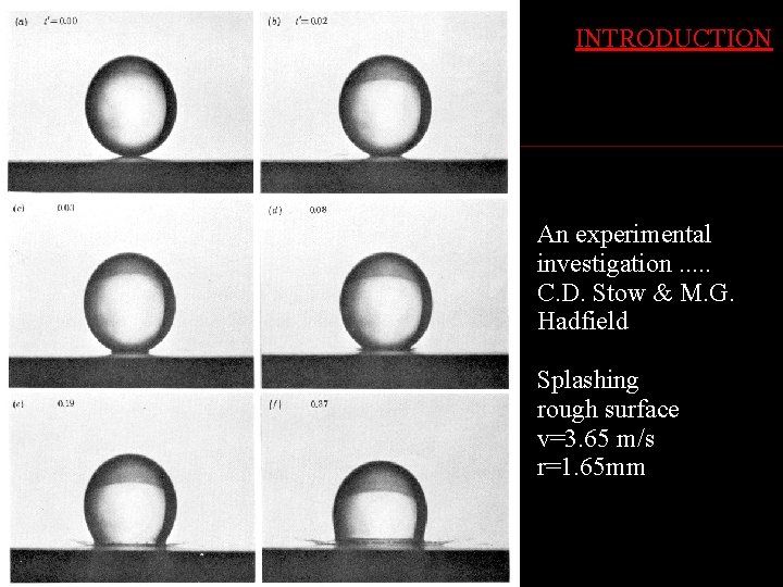
INTRODUCTION An experimental investigation. . . C. D. Stow & M. G. Hadfield Splashing rough surface v=3. 65 m/s r=1. 65 mm

INTRODUCTION 1) Problem : Numerical Representation of Interfaces An experimental • Impact Dynamics : solid surface + liquid interface = drop surface • Splash Dynamics : liquid interface -> more liquid interfaces 2) Problem : Correct Physics • Impact Dynamics : solid surface + liquid interface = drop surface • Splash Dynamics : liquid interface -> more liquid interfaces Hypoteses: No simulation of the impact No splash o total rebound (low Re numbers, no rough surfaces) Axisymmetric simulation Numerical Representation of Interfaces -> ok Correct Physics ?

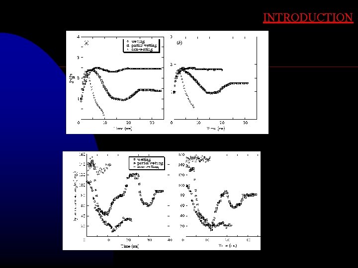
INTRODUCTION Some features: • Behavior of the impact for: Wettable-P/Wettable N/Wettable surfaces • • Deposition – Partial rebound – total rebound • Surface capillary waves • Spreading ratio and Max spreading ratio • Static/Dynamic/apparent Contact angle

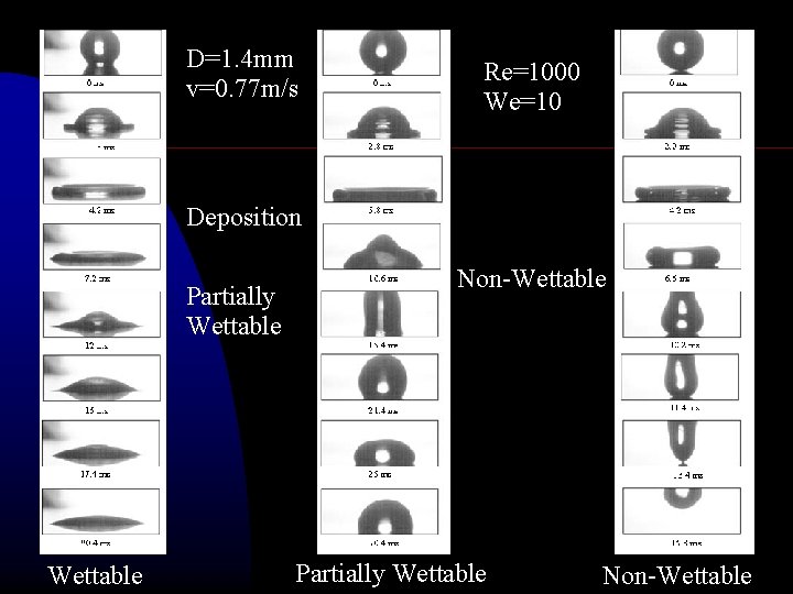
D=1. 4 mm v=0. 77 m/s Re=1000 We=10 Deposition Partially Wettable Non-Wettable

INTRODUCTION

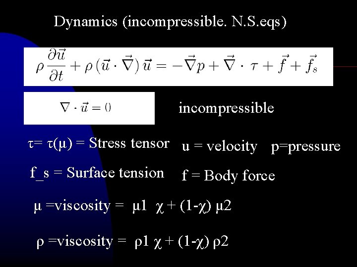
Dynamics (incompressible. N. S. eqs) incompressible τ= τ(μ) = Stress tensor u = velocity p=pressure f_s = Surface tension f = Body force μ =viscosity = μ 1 χ + (1 -χ) μ 2 ρ =viscosity = ρ1 χ + (1 -χ) ρ2

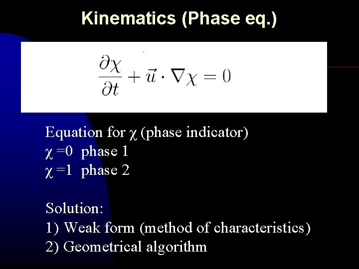
Kinematics (Phase eq. ) Equation for χ (phase indicator) χ =0 phase 1 χ =1 phase 2 Solution: 1) Weak form (method of characteristics) 2) Geometrical algorithm

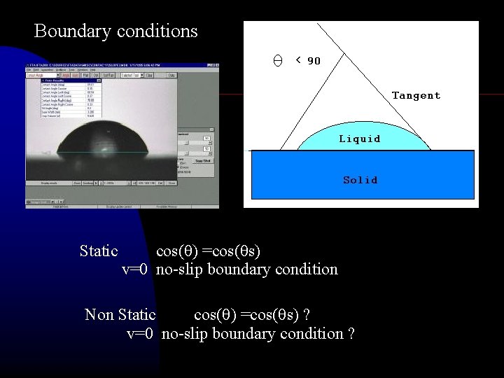
Boundary conditions Static cos( ) =cos( s) v=0 no-slip boundary condition Non Static cos( ) =cos( s) ? v=0 no-slip boundary condition ?

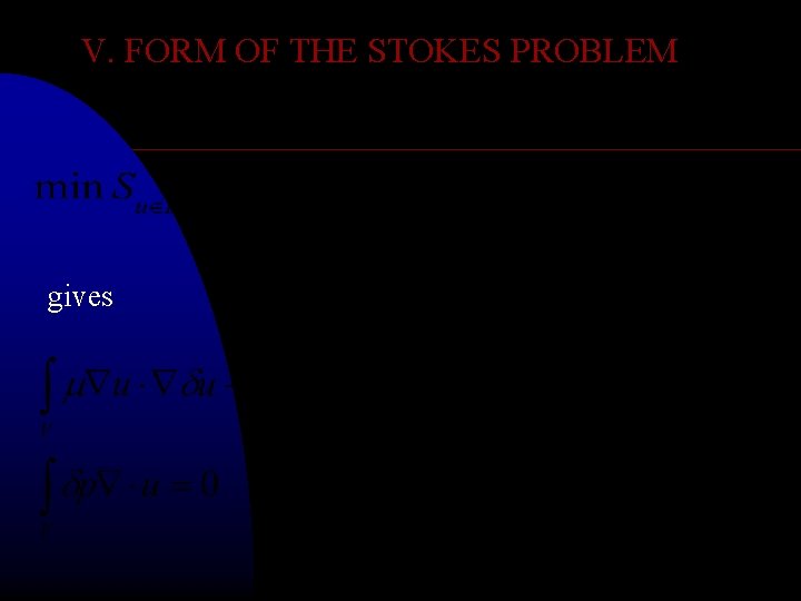
V. FORM OF THE STOKES PROBLEM gives

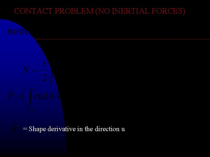
CONTACT PROBLEM (NO INERTIAL FORCES) = Shape derivative in the direction u

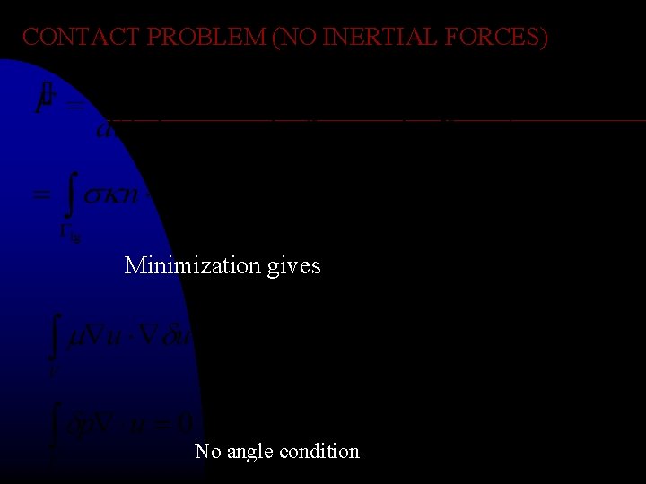
CONTACT PROBLEM (NO INERTIAL FORCES) Minimization gives No angle condition

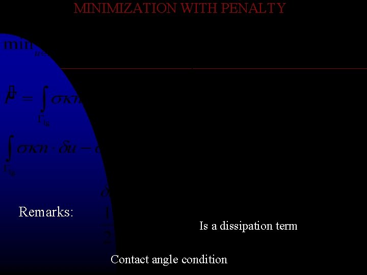
MINIMIZATION WITH PENALTY Remarks: Is a dissipation term Contact angle condition

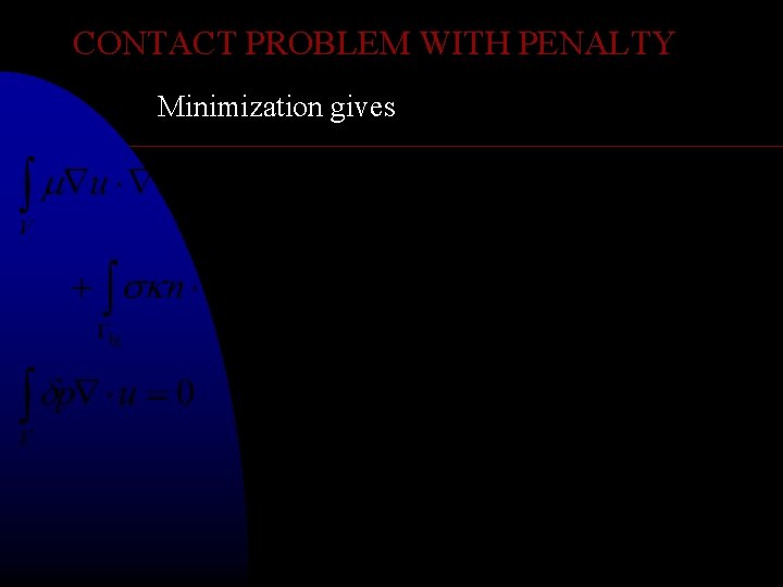
CONTACT PROBLEM WITH PENALTY Minimization gives

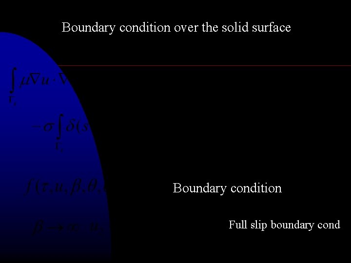
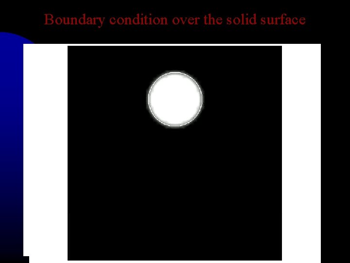
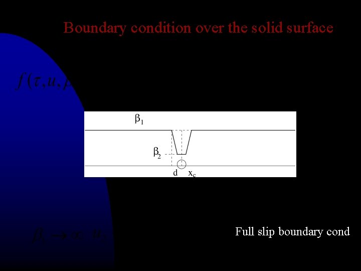
Boundary condition over the solid surface Boundary condition Full slip boundary cond

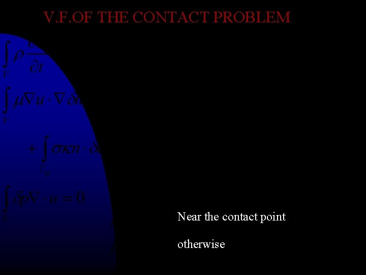
V. F. OF THE CONTACT PROBLEM Near the contact point otherwise

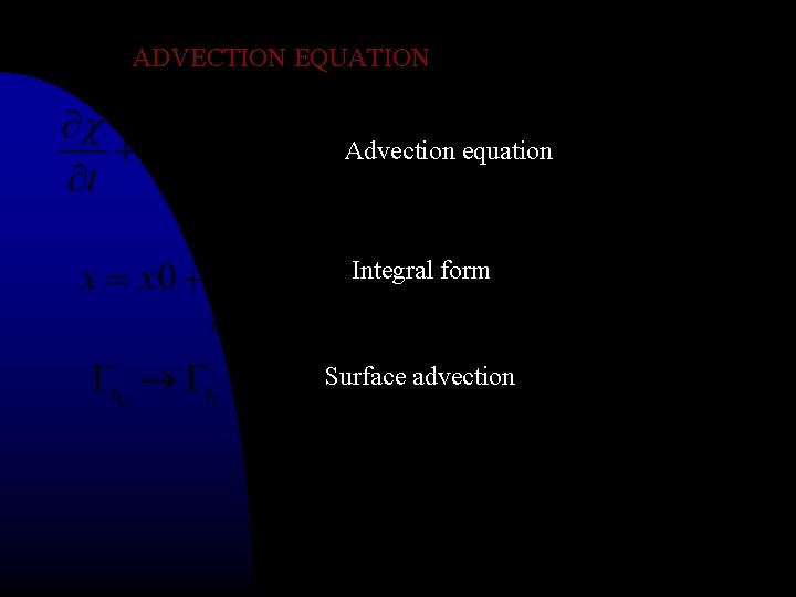
Numerical solution Fem solution • Weak form -> fem • Advection equation -> integral form • Density and viscosity are discountinuous -> weak f. • Surface term singularity-> weak form

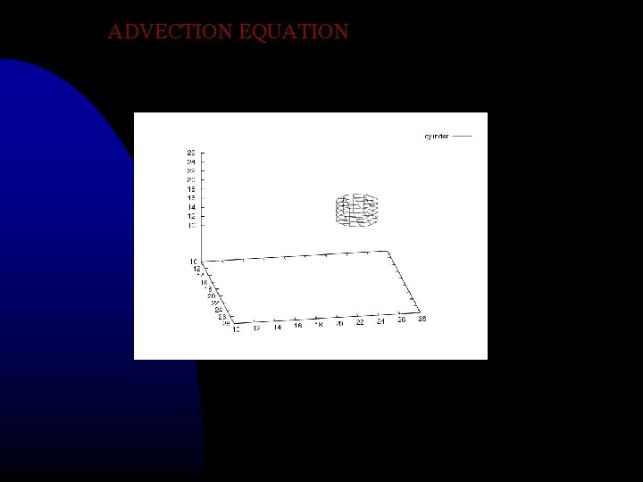
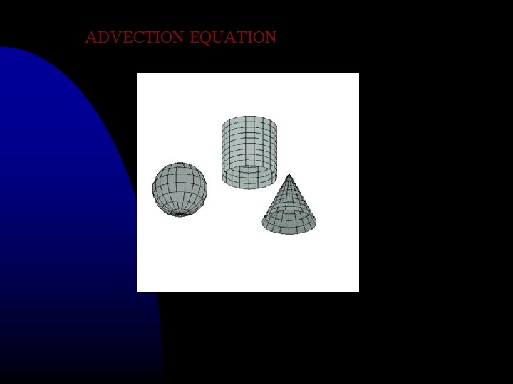
ADVECTION EQUATION Advection equation Integral form Surface advection

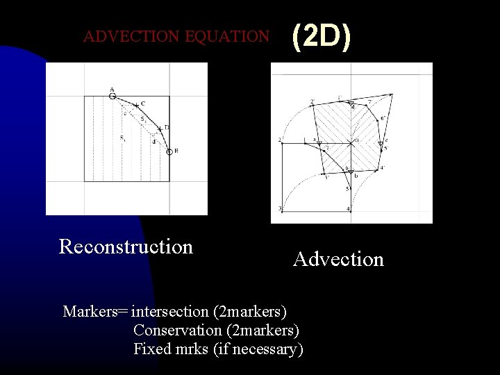
ADVECTION EQUATION Reconstruction (2 D) Advection Markers= intersection (2 markers) Conservation (2 markers) Fixed mrks (if necessary)

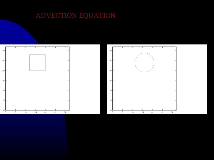
ADVECTION EQUATION

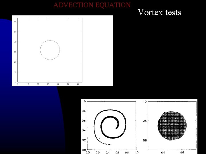
ADVECTION EQUATION Vortex tests

ADVECTION EQUATION

ADVECTION EQUATION

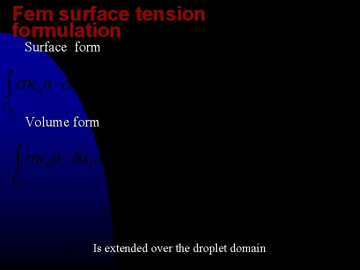
Fem surface tension formulation Surface form Volume form Is extended over the droplet domain

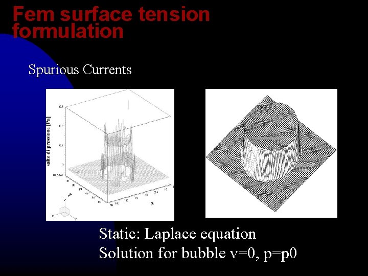
Fem surface tension formulation Spurious Currents Static: Laplace equation Solution for bubble v=0, p=p 0

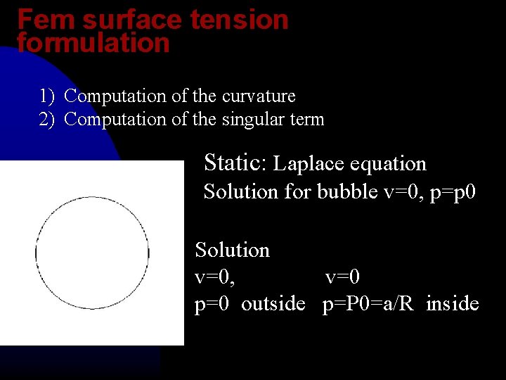
Fem surface tension formulation 1) Computation of the curvature 2) Computation of the singular term Static: Laplace equation Solution for bubble v=0, p=p 0 Solution v=0, v=0 p=0 outside p=P 0=a/R inside

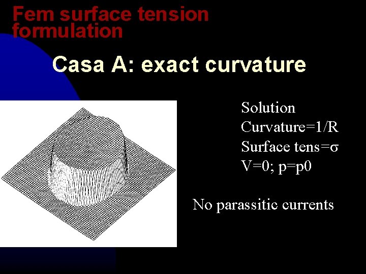
Fem surface tension formulation Casa A: exact curvature Solution Curvature=1/R Surface tens=σ V=0; p=p 0 No parassitic currents

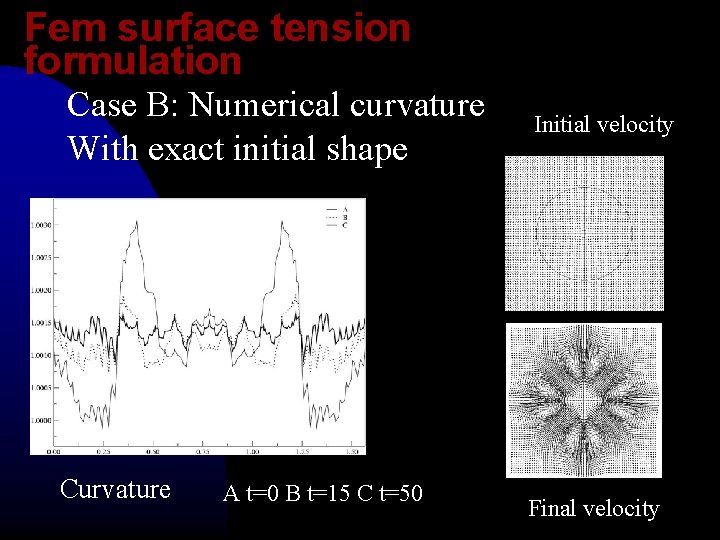
Fem surface tension formulation Case B: Numerical curvature With exact initial shape Curvature A t=0 B t=15 C t=50 Initial velocity Final velocity

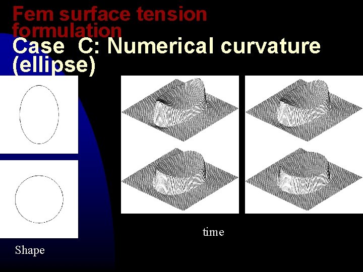
Fem surface tension formulation Case C: Numerical curvature (ellipse) time Shape

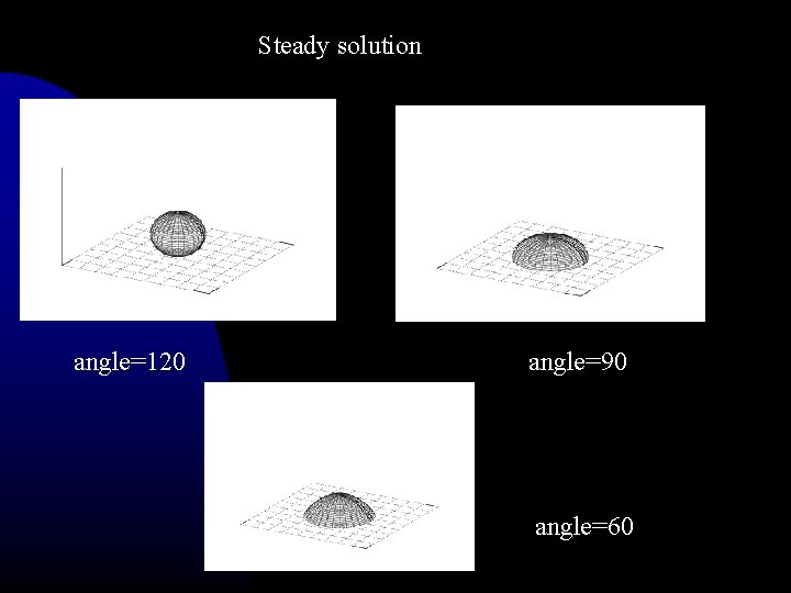
Steady solution angle=120 angle=90 angle=60

Boundary condition over the solid surface

Boundary condition over the solid surface Full slip boundary cond

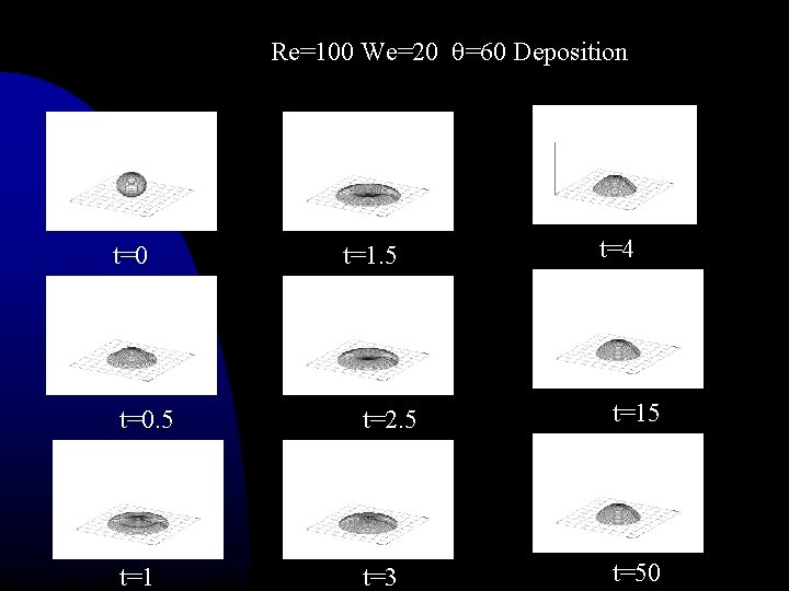
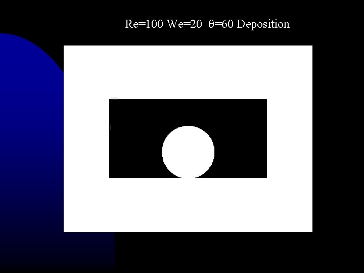
Re=100 We=20 =60 Deposition t=0 t=1. 5 t=4 t=0 t=0. 5 t=2. 5 t=15 t=3 t=50 t=1

Re=100 We=20 =60 Deposition

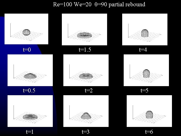
Re=100 We=20 =90 partial rebound t=0 t=1. 5 t=0 t=0. 5 t=1 t=2 t=3 t=4 t=0 t=5 t=6

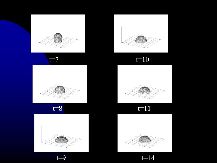
t=7 t=8 t=9 t=10 t=11 t=14

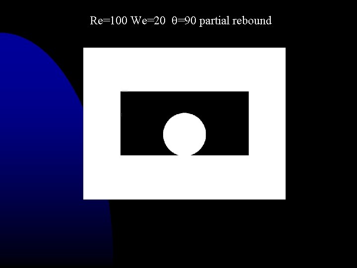
Re=100 We=20 =90 partial rebound

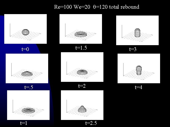
Re=100 We=20 =120 total rebound t=1. 5 t=0 t=2 t=. 5 t=7 t=1 t=2. 5 t=3 t=4

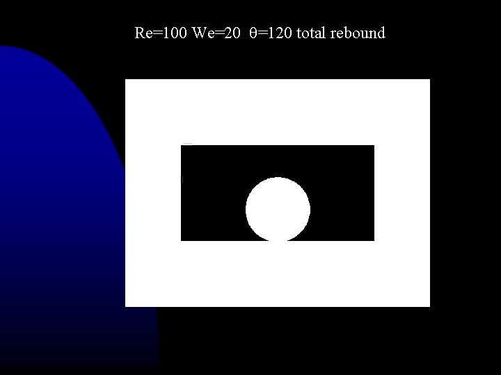
Re=100 We=20 =120 total rebound

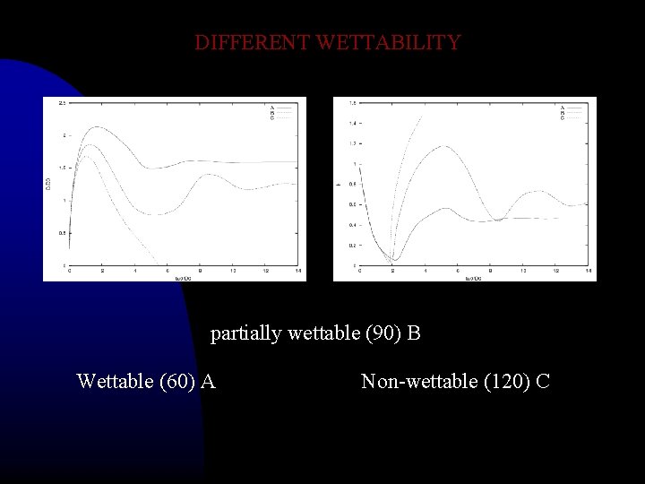
DIFFERENT WETTABILITY partially wettable (90) B Wettable (60) A Non-wettable (120) C

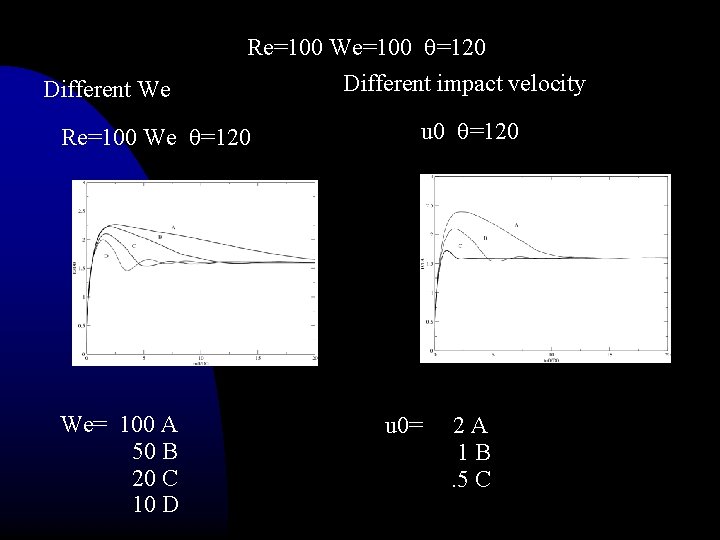
Re=100 We=100 =120 Different We Re=100 We =120 We= 100 A 50 B 20 C 10 D Different impact velocity u 0 =120 u 0= 2 A 1 B. 5 C

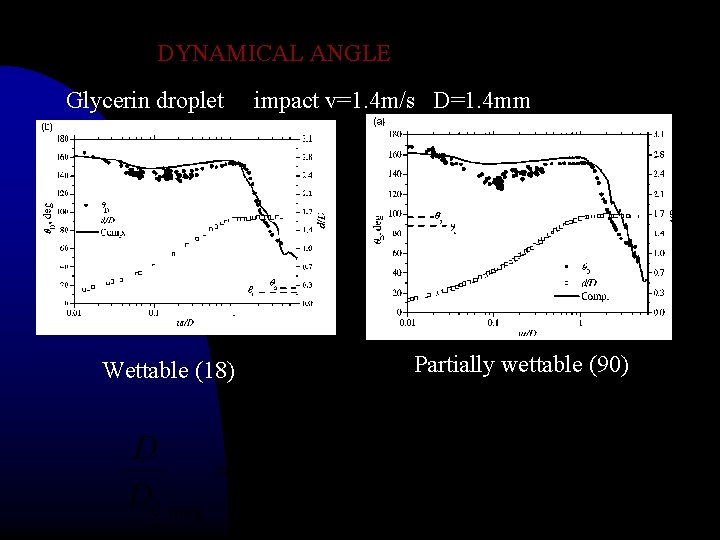
DYNAMICAL ANGLE Glycerin droplet Wettable (18) impact v=1. 4 m/s D=1. 4 mm Partially wettable (90)

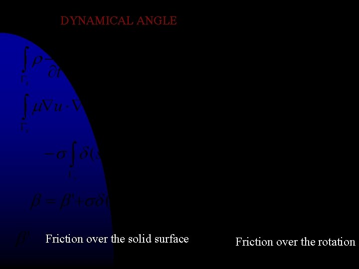
DYNAMICAL ANGLE Friction over the solid surface Friction over the rotation

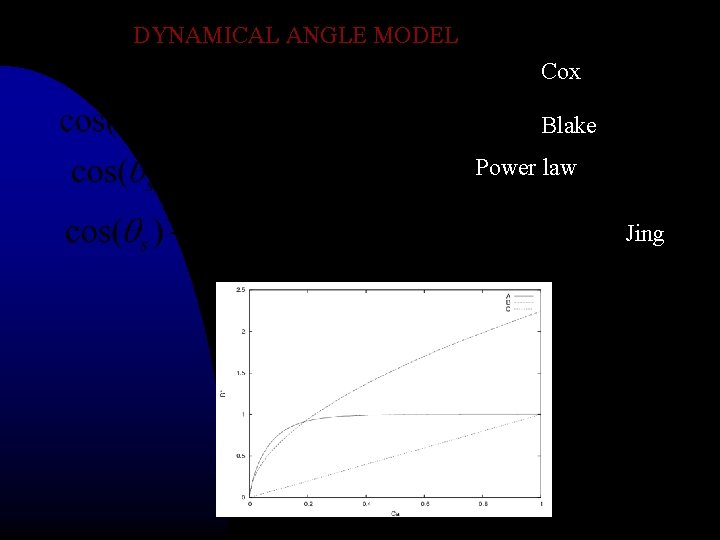
DYNAMICAL ANGLE MODEL Cox Blake Power law Jing

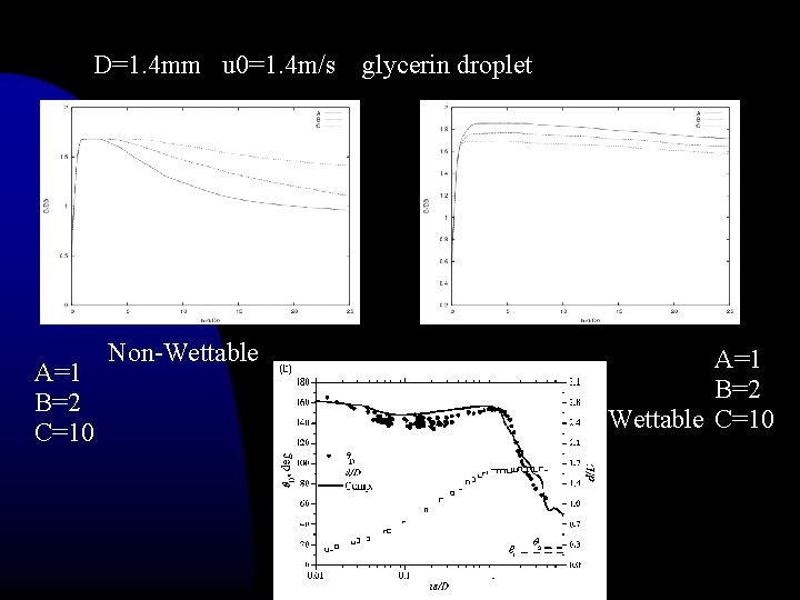
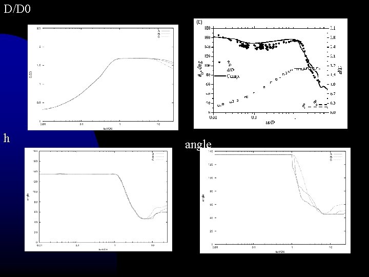
D=1. 4 mm u 0=1. 4 m/s A=1 B=2 C=10 Non-Wettable glycerin droplet A=1 B=2 Wettable C=10

D/D 0 h angle

Conclusions - Variational contact models can be used - Open question: Can we simulate large classes • of droplet impacts with a unique setting of • boundary conditions ?

Thanks