Variational Inference and Variational Message Passing John Winn

Variational Inference and Variational Message Passing John Winn Microsoft Research, Cambridge 12 th November 2004 Robotics Research Group, University of Oxford

Overview n Probabilistic models & Bayesian inference n Variational Inference n Variational Message Passing n Vision example

Overview n Probabilistic models & Bayesian inference n Variational Inference n Variational Message Passing n Vision example

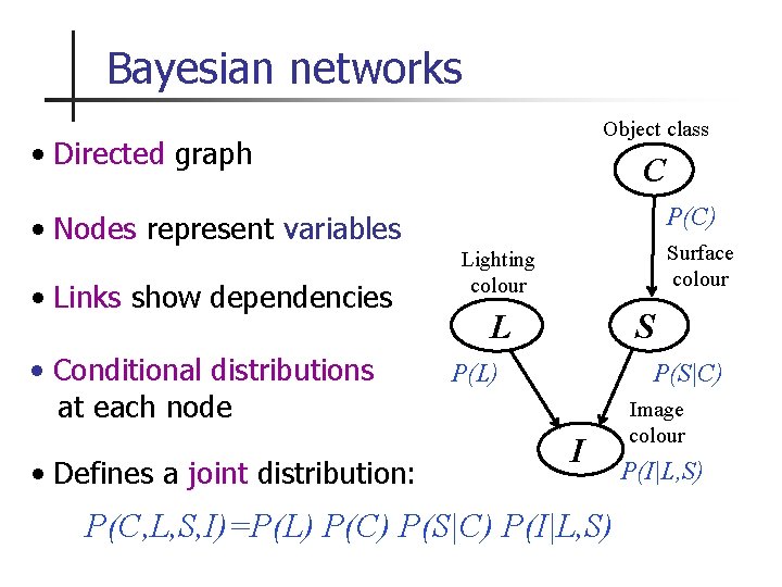
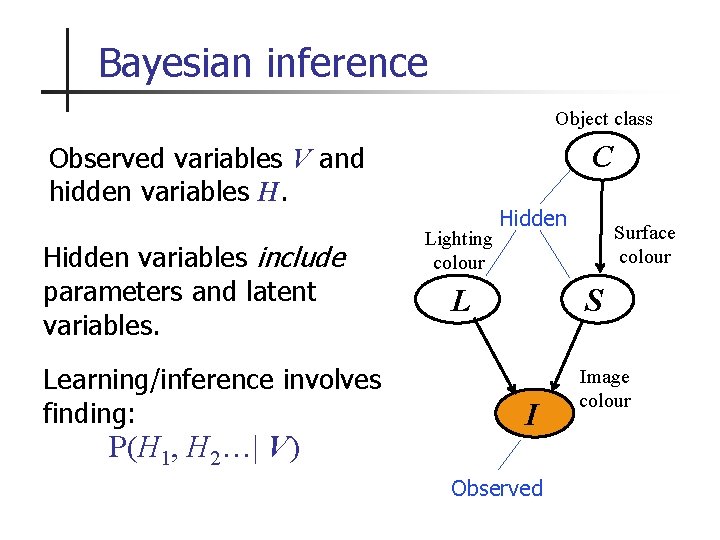
Bayesian networks Object class • Directed graph C P(C) • Nodes represent variables • Links show dependencies • Conditional distributions at each node • Defines a joint distribution: Surface colour Lighting colour L S P(L) P(S|C) I P(C, L, S, I)=P(L) P(C) P(S|C) P(I|L, S) Image colour P(I|L, S)

Bayesian inference Object class C Observed variables V and hidden variables H. Hidden variables include parameters and latent variables. Learning/inference involves finding: P(H 1, H 2…| V) Lighting colour Hidden L Surface colour S I Observed Image colour

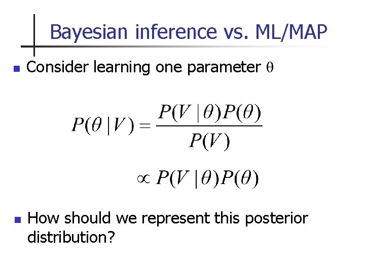
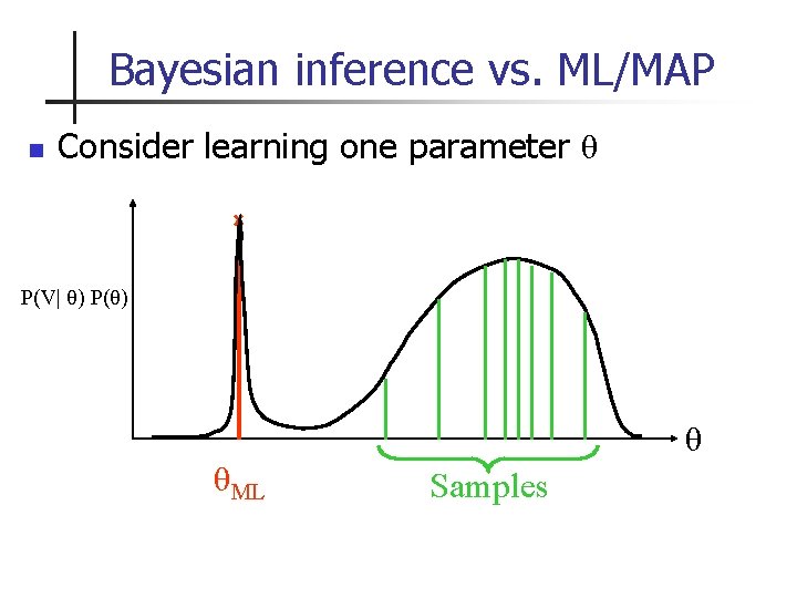
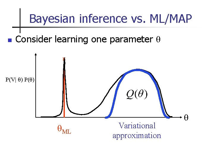
Bayesian inference vs. ML/MAP n n Consider learning one parameter θ How should we represent this posterior distribution?

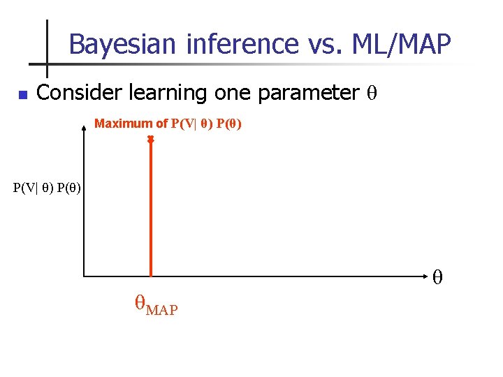
Bayesian inference vs. ML/MAP n Consider learning one parameter θ Maximum of P(V| θ) P(θ) θ θMAP

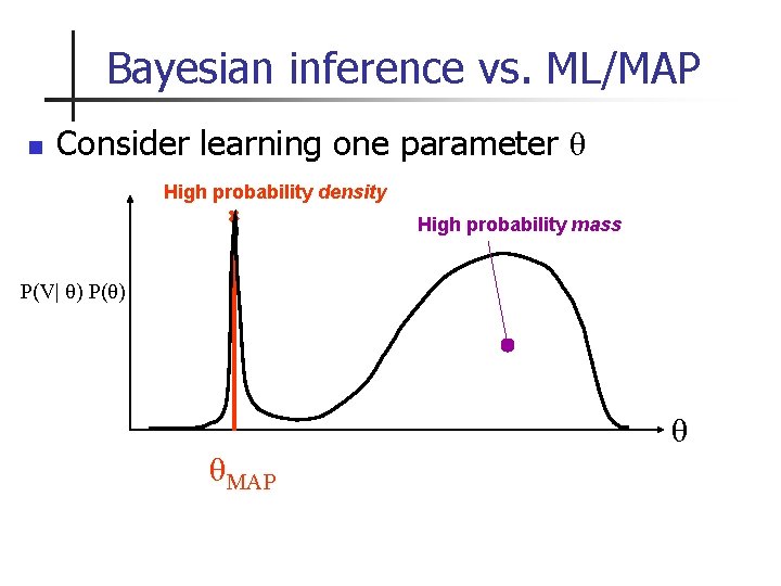
Bayesian inference vs. ML/MAP n Consider learning one parameter θ High probability density High probability mass P(V| θ) P(θ) θ θMAP

Bayesian inference vs. ML/MAP n Consider learning one parameter θ P(V| θ) P(θ) θ θML Samples

Bayesian inference vs. ML/MAP n Consider learning one parameter θ P(V| θ) P(θ) θML Variational approximation θ

Overview n Probabilistic models & Bayesian inference n Variational Inference n Variational Message Passing n Vision example

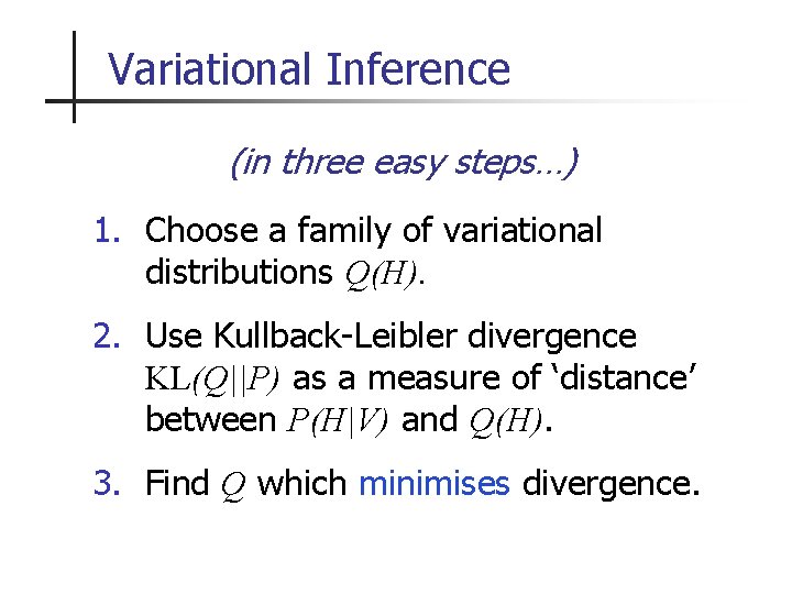
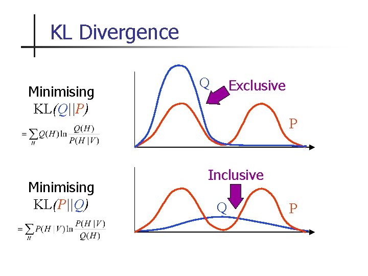
Variational Inference (in three easy steps…) 1. Choose a family of variational distributions Q(H). 2. Use Kullback-Leibler divergence KL(Q||P) as a measure of ‘distance’ between P(H|V) and Q(H). 3. Find Q which minimises divergence.

KL Divergence Minimising KL(Q||P) Minimising KL(P||Q) Q Exclusive P Inclusive Q P

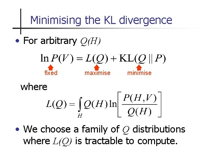
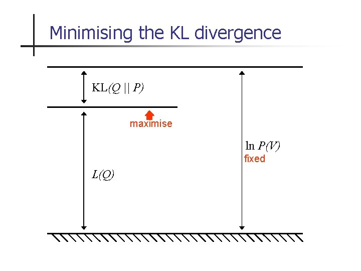
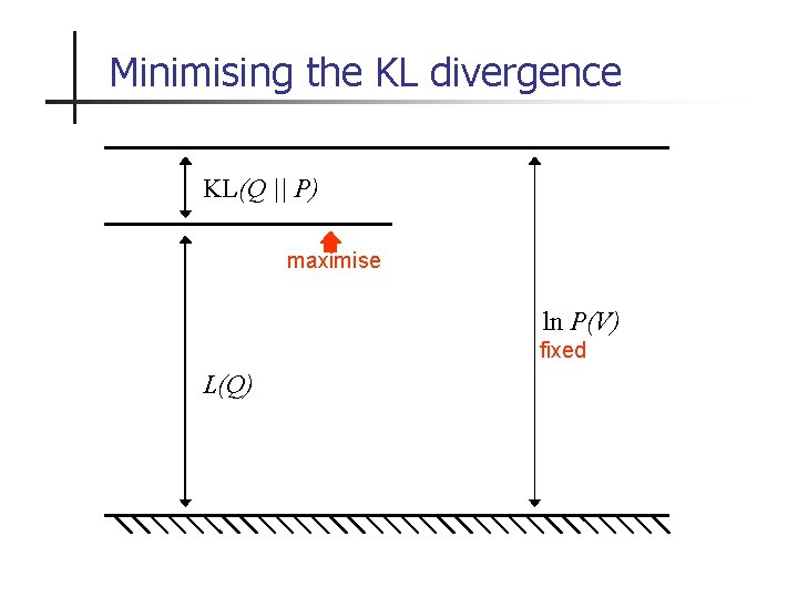
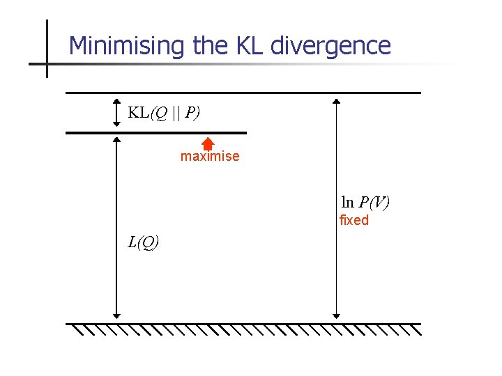
Minimising the KL divergence • For arbitrary Q(H) fixed maximise minimise where • We choose a family of Q distributions where L(Q) is tractable to compute.

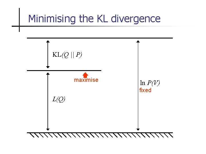
Minimising the KL divergence KL(Q || P) maximise ln P(V) fixed L(Q)

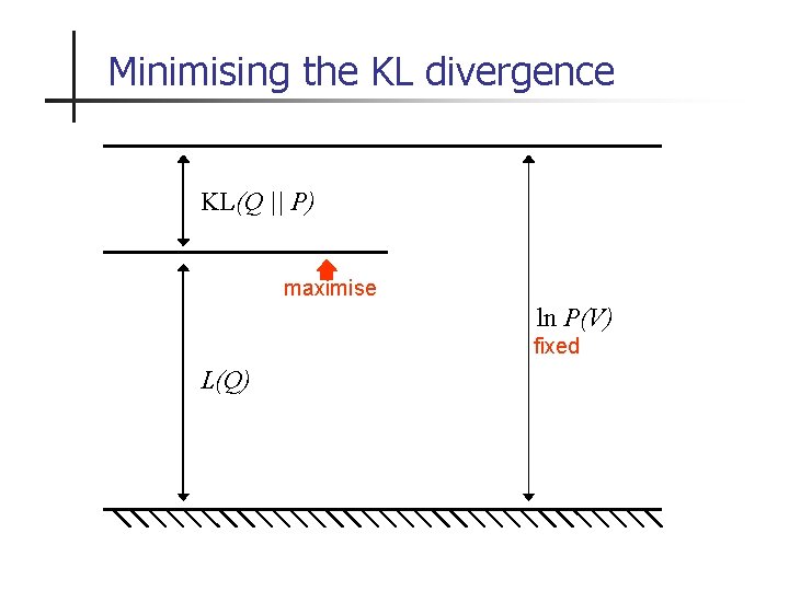
Minimising the KL divergence KL(Q || P) maximise ln P(V) fixed L(Q)

Minimising the KL divergence KL(Q || P) maximise ln P(V) fixed L(Q)

Minimising the KL divergence KL(Q || P) maximise ln P(V) fixed L(Q)

Minimising the KL divergence KL(Q || P) maximise ln P(V) fixed L(Q)

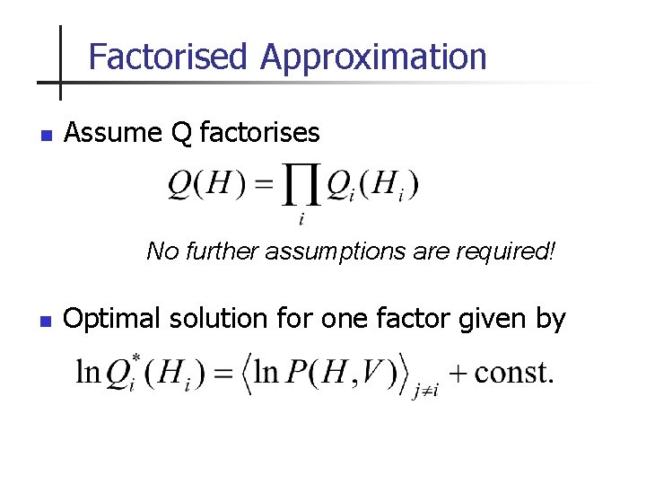
Factorised Approximation n Assume Q factorises No further assumptions are required! n Optimal solution for one factor given by

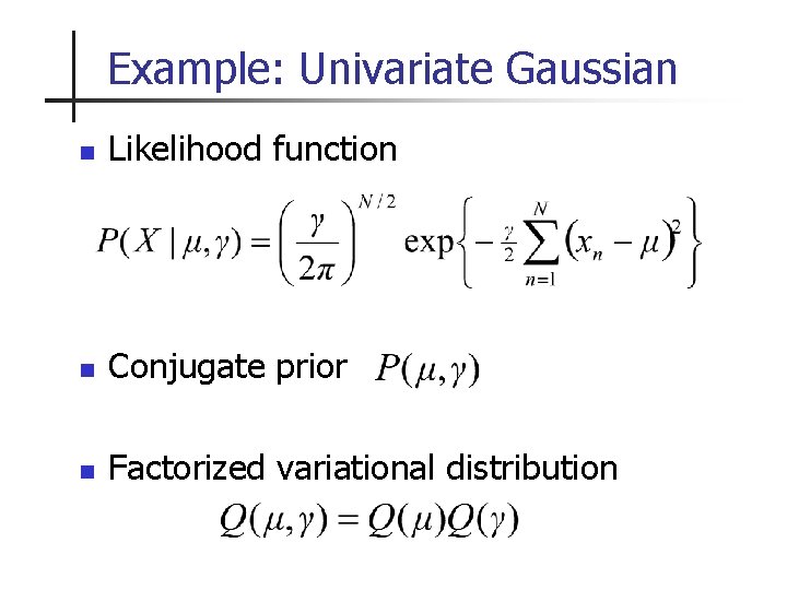
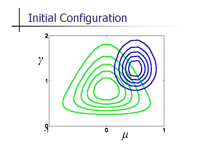
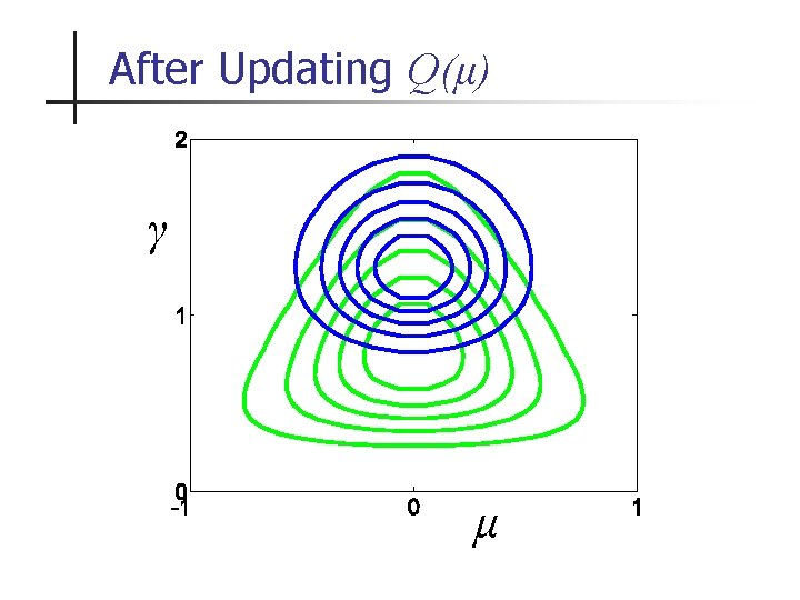
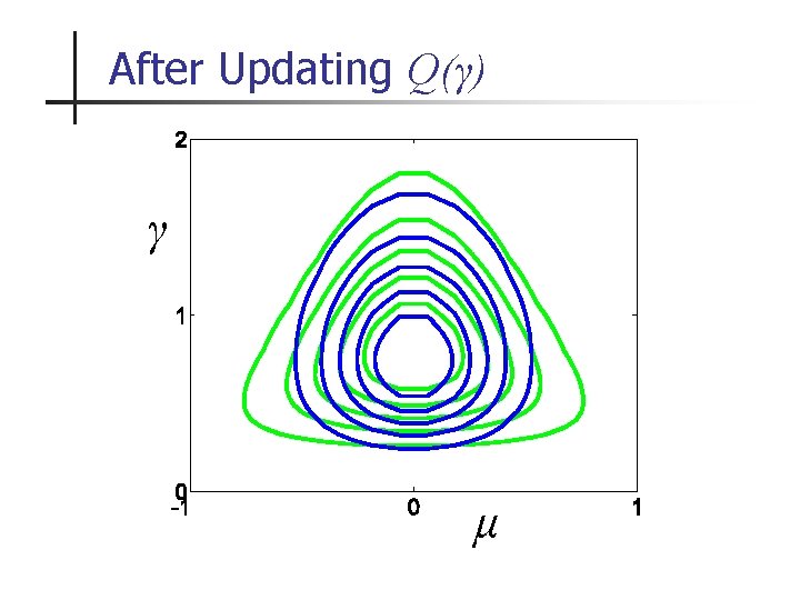
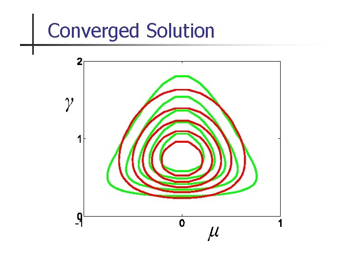
Example: Univariate Gaussian n Likelihood function n Conjugate prior n Factorized variational distribution

Initial Configuration γ μ

After Updating Q(μ) γ μ

After Updating Q(γ) γ μ

Converged Solution γ μ

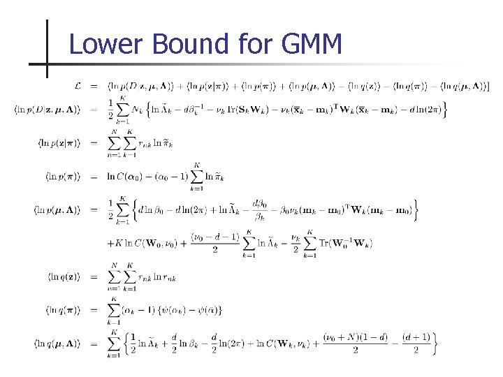
Lower Bound for GMM

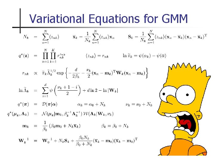
Variational Equations for GMM

Overview n Probabilistic models & Bayesian inference n Variational Inference n Variational Message Passing n Vision example

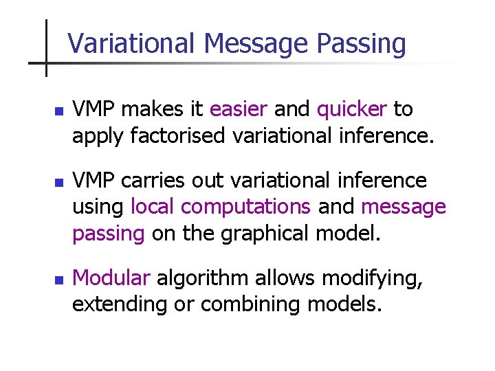
Variational Message Passing n n n VMP makes it easier and quicker to apply factorised variational inference. VMP carries out variational inference using local computations and message passing on the graphical model. Modular algorithm allows modifying, extending or combining models.

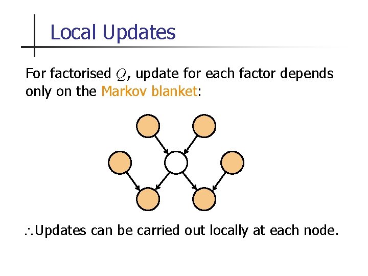
Local Updates For factorised Q, update for each factor depends only on the Markov blanket: Updates can be carried out locally at each node.

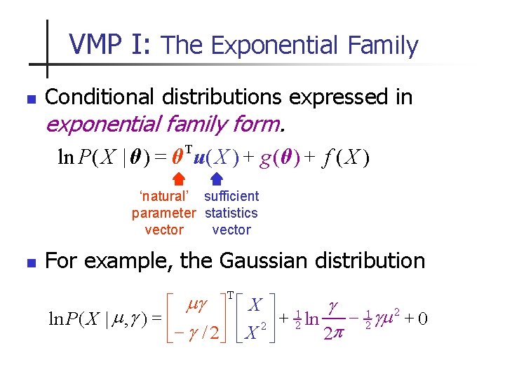
VMP I: The Exponential Family n Conditional distributions expressed in exponential family form. T = ln P( X | θ ) θ u( X ) + g (θ ) + f ( X ) ‘natural’ sufficient parameter statistics vector n For example, the Gaussian distribution é mg ù é X ù 1 gm 2 + + ln P( X | m , g ) = ê ln 0 ú ê 2 2 2ú 2 p ë - g / 2û ë X û T

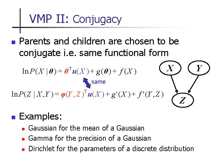
VMP II: Conjugacy n Parents and children are chosen to be conjugate i. e. same functional form ln P ( X | θ ) = θ T u( X ) + g (θ ) + f ( X ) X Y same T = ln P( Z | X , Y ) φ(Y , Z ) u( X ) + g ' ( X ) + f ' (Y , Z ) n Z Examples: n n n Gaussian for the mean of a Gaussian Gamma for the precision of a Gaussian Dirichlet for the parameters of a discrete distribution

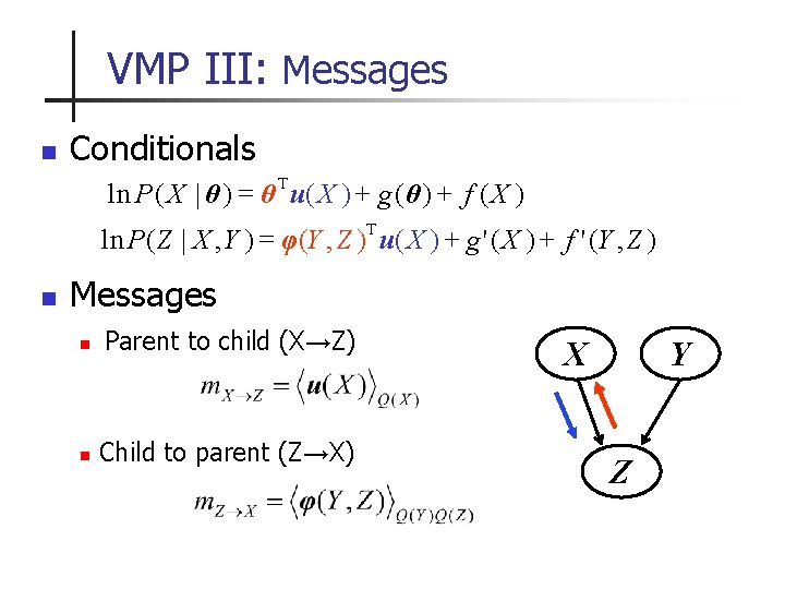
VMP III: Messages n Conditionals ln P ( X | θ ) = θ T u( X ) + g (θ ) + f ( X ) T = ln P( Z | X , Y ) φ(Y , Z ) u( X ) + g ' ( X ) + f ' (Y , Z ) n Messages n Parent to child (X→Z) n Child to parent (Z→X) X Y Z

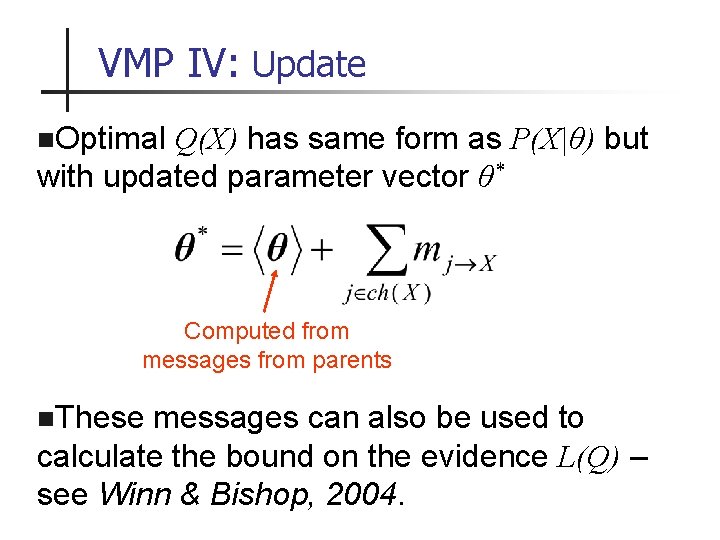
VMP IV: Update n. Optimal Q(X) has same form as P(X|θ) but with updated parameter vector θ* Computed from messages from parents n. These messages can also be used to calculate the bound on the evidence L(Q) – see Winn & Bishop, 2004.

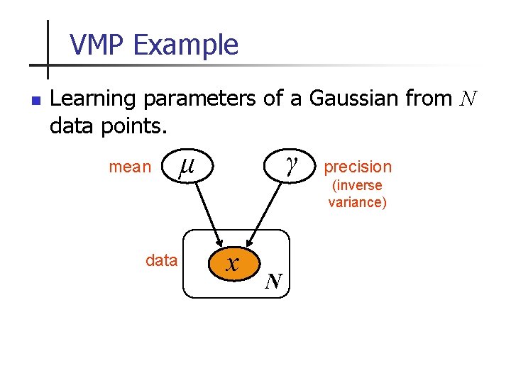
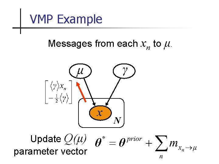
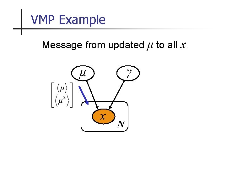
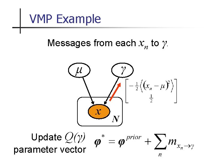
VMP Example n Learning parameters of a Gaussian from N data points. mean data γ μ precision (inverse variance) x N

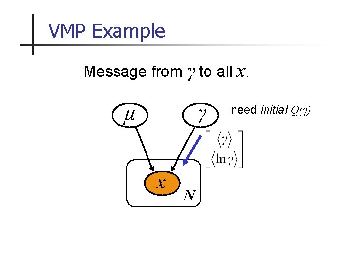
VMP Example Message from γ to all x. γ μ x N need initial Q(γ)

VMP Example Messages from each xn to μ. γ μ x Update Q(μ) parameter vector N

VMP Example Message from updated μ to all x. γ μ x N

VMP Example Messages from each xn to γ. γ μ x Update Q(γ) parameter vector N

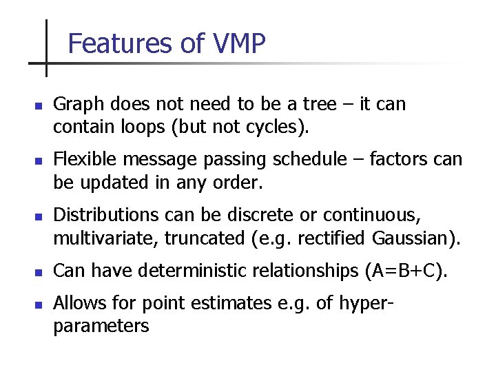
Features of VMP n n n Graph does not need to be a tree – it can contain loops (but not cycles). Flexible message passing schedule – factors can be updated in any order. Distributions can be discrete or continuous, multivariate, truncated (e. g. rectified Gaussian). Can have deterministic relationships (A=B+C). Allows for point estimates e. g. of hyperparameters

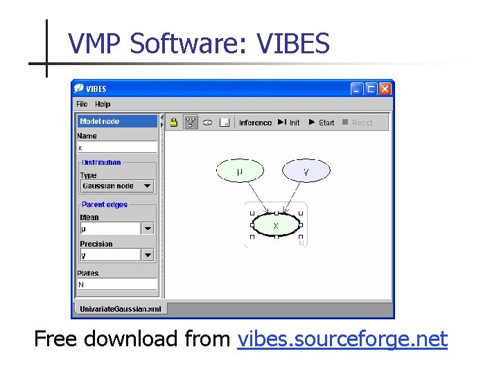
VMP Software: VIBES Free download from vibes. sourceforge. net

Overview n Probabilistic models & Bayesian inference n Variational Inference n Variational Message Passing n Vision example

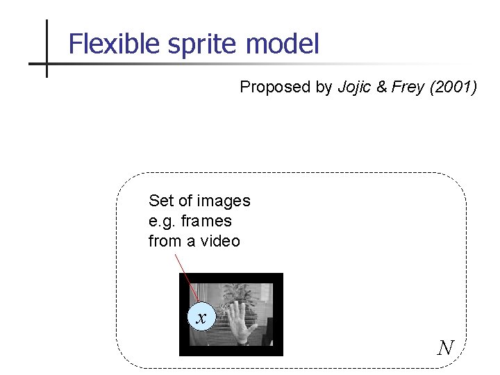
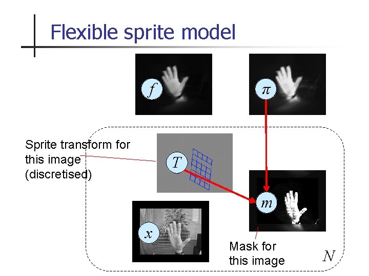
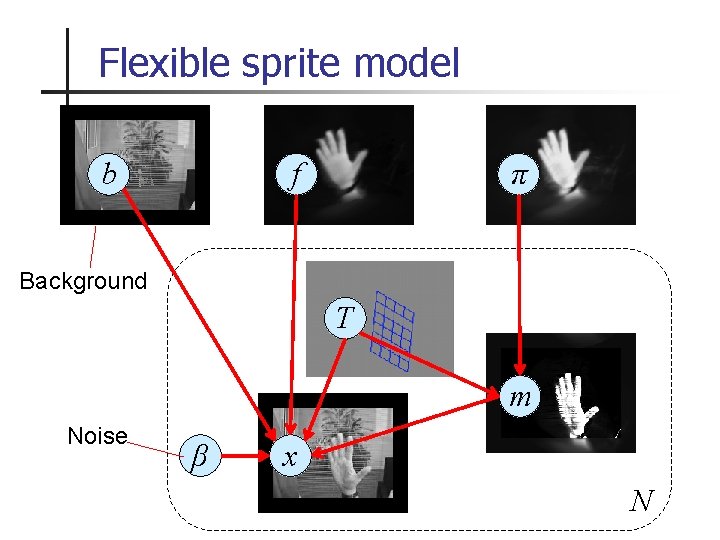
Flexible sprite model Proposed by Jojic & Frey (2001) Set of images e. g. frames from a video x N

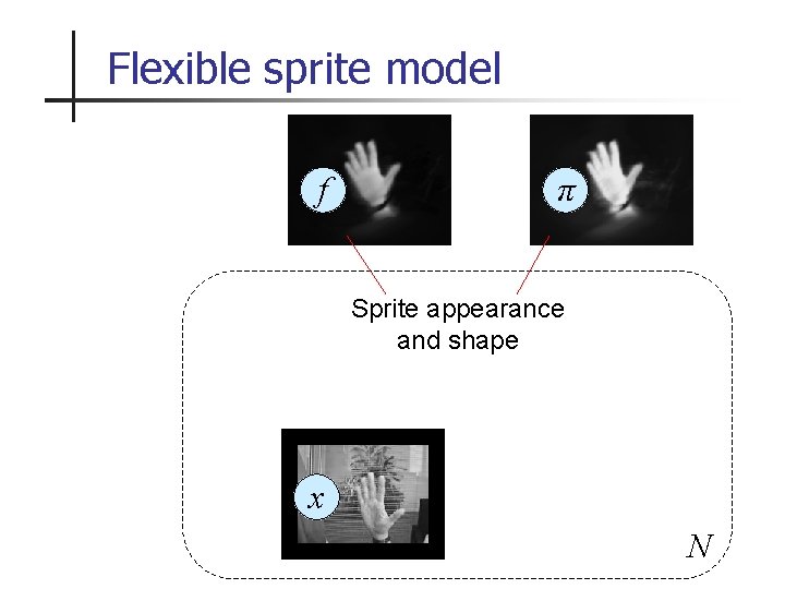
Flexible sprite model f π Sprite appearance and shape x N

Flexible sprite model f Sprite transform for this image (discretised) π T m x Mask for this image N

Flexible sprite model b f π Background T m Noise β x N

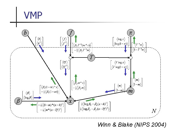
VMP b π f T m β x N Winn & Blake (NIPS 2004)

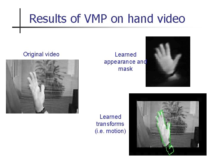
Results of VMP on hand video Original video Learned appearance and mask Learned transforms (i. e. motion)

Conclusions n n n Variational Message Passing allows approximate Bayesian inference for a wide range of models. VMP simplifies the construction, testing, extension and comparison of models. You can try VMP for yourself vibes. sourceforge. net

That’s all folks!