Artificial Neural Networks Dr Lahouari Ghouti Information Computer

Artificial Neural Networks Dr. Lahouari Ghouti Information & Computer Science Department Artificial Neural Networks

Single-Layer Perceptron (SLP) Artificial Neural Networks

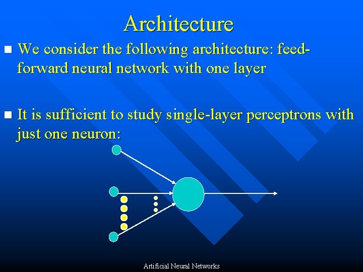
Architecture n We consider the following architecture: feedforward neural network with one layer n It is sufficient to study single-layer perceptrons with just one neuron: Artificial Neural Networks

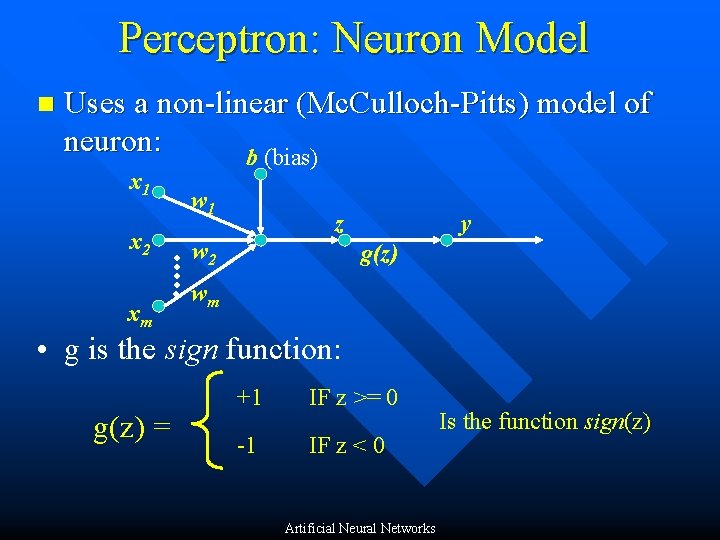
Perceptron: Neuron Model n Uses a non-linear (Mc. Culloch-Pitts) model of neuron: b (bias) x 1 x 2 xm w 1 z w 2 y g(z) wm • g is the sign function: g(z) = +1 IF z >= 0 -1 IF z < 0 Artificial Neural Networks Is the function sign(z)

Perceptron: Applications n The perceptron is used for classification (? ): classify correctly a set of examples into one of the two classes C 1, C 2: n If the output of the perceptron is +1 then the input is assigned to class C 1 n If the output is -1 then the input is assigned to C 2 Artificial Neural Networks

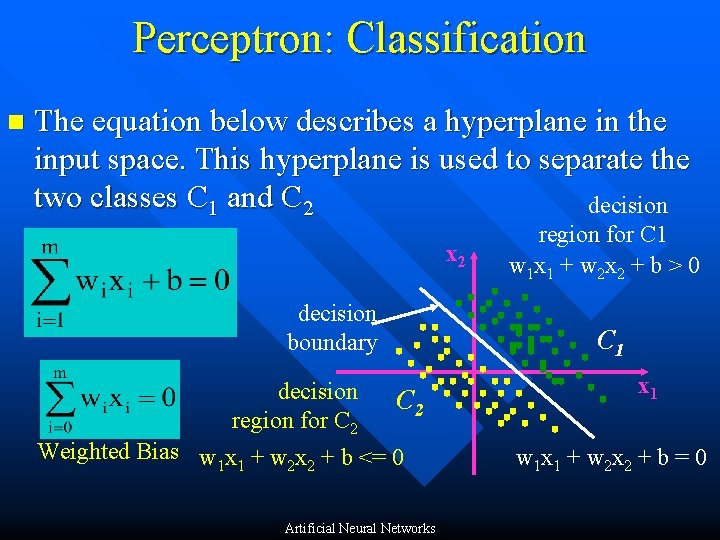
Perceptron: Classification n The equation below describes a hyperplane in the input space. This hyperplane is used to separate the two classes C 1 and C 2 decision x 2 decision boundary decision region for C 2 region for C 1 w 1 x 1 + w 2 x 2 + b > 0 C 1 C 2 Weighted Bias w 1 x 1 + w 2 x 2 + b <= 0 Artificial Neural Networks x 1 w 1 x 1 + w 2 x 2 + b = 0

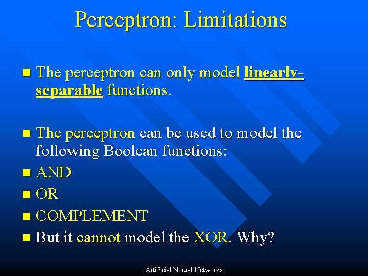
Perceptron: Limitations n The perceptron can only model linearlyseparable functions. The perceptron can be used to model the following Boolean functions: n AND n OR n COMPLEMENT n But it cannot model the XOR. Why? n Artificial Neural Networks

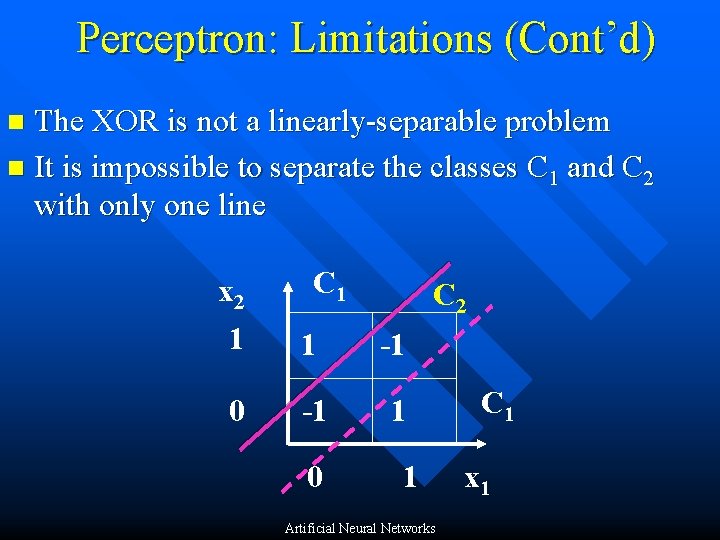
Perceptron: Limitations (Cont’d) The XOR is not a linearly-separable problem n It is impossible to separate the classes C 1 and C 2 with only one line n C 1 x 2 1 1 -1 0 -1 1 0 C 2 1 Artificial Neural Networks C 1 x 1

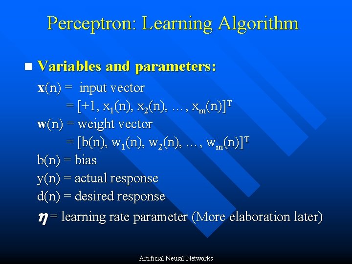
Perceptron: Learning Algorithm n Variables and parameters: x(n) = input vector = [+1, x 1(n), x 2(n), …, xm(n)]T w(n) = weight vector = [b(n), w 1(n), w 2(n), …, wm(n)]T b(n) = bias y(n) = actual response d(n) = desired response = learning rate parameter (More elaboration later) Artificial Neural Networks

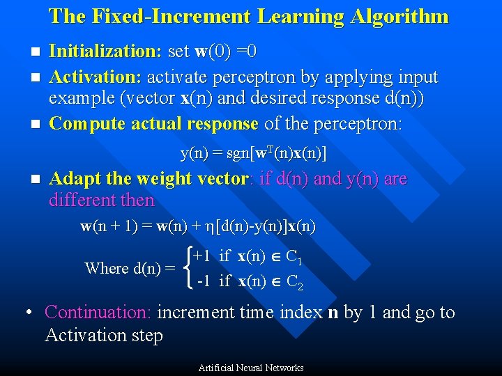
The Fixed-Increment Learning Algorithm n n n Initialization: set w(0) =0 Activation: activate perceptron by applying input example (vector x(n) and desired response d(n)) Compute actual response of the perceptron: y(n) = sgn[w. T(n)x(n)] n Adapt the weight vector: if d(n) and y(n) are different then w(n + 1) = w(n) + [d(n)-y(n)]x(n) Where d(n) = +1 if x(n) C 1 -1 if x(n) C 2 • Continuation: increment time index n by 1 and go to Activation step Artificial Neural Networks

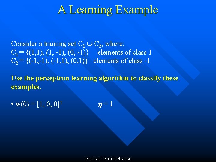
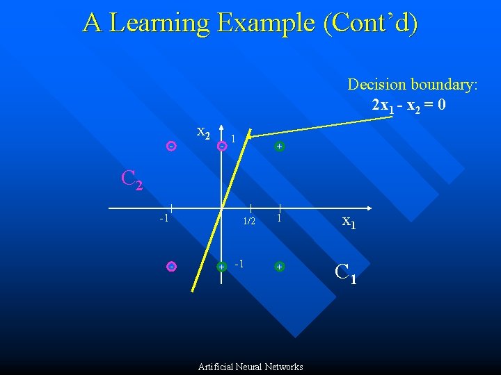
A Learning Example Consider a training set C 1 C 2, where: C 1 = {(1, 1), (1, -1), (0, -1)} elements of class 1 C 2 = {(-1, -1), (-1, 1), (0, 1)} elements of class -1 Use the perceptron learning algorithm to classify these examples. • w(0) = [1, 0, 0]T =1 Artificial Neural Networks

A Learning Example (Cont’d) Decision boundary: 2 x 1 - x 2 = 0 - x 2 - 1 + C 2 -1 1/2 - + -1 1 x 1 + C 1 Artificial Neural Networks

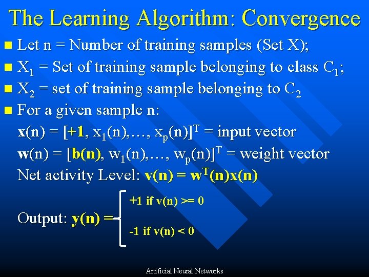
The Learning Algorithm: Convergence Let n = Number of training samples (Set X); n X 1 = Set of training sample belonging to class C 1; n X 2 = set of training sample belonging to C 2 n For a given sample n: x(n) = [+1, x 1(n), …, xp(n)]T = input vector w(n) = [b(n), w 1(n), …, wp(n)]T = weight vector Net activity Level: v(n) = w. T(n)x(n) n +1 if v(n) >= 0 Output: y(n) = -1 if v(n) < 0 Artificial Neural Networks

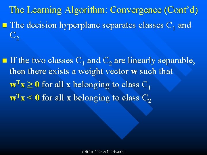
The Learning Algorithm: Convergence (Cont’d) n The decision hyperplane separates classes C 1 and C 2 n If the two classes C 1 and C 2 are linearly separable, then there exists a weight vector w such that w. Tx ≥ 0 for all x belonging to class C 1 w. Tx < 0 for all x belonging to class C 2 Artificial Neural Networks

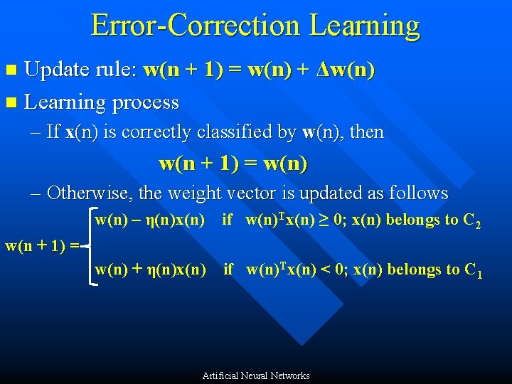
Error-Correction Learning Update rule: w(n + 1) = w(n) + Δw(n) n Learning process n – If x(n) is correctly classified by w(n), then w(n + 1) = w(n) – Otherwise, the weight vector is updated as follows w(n) – η(n)x(n) if w(n)Tx(n) ≥ 0; x(n) belongs to C 2 w(n + 1) = w(n) + η(n)x(n) if w(n)Tx(n) < 0; x(n) belongs to C 1 Artificial Neural Networks

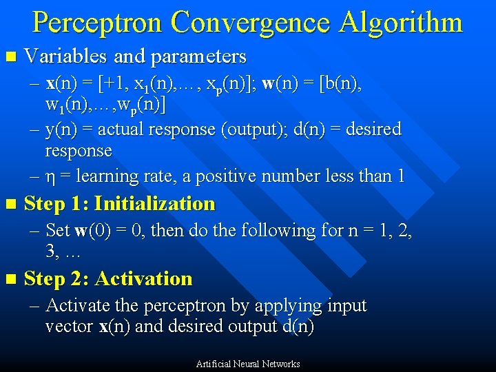
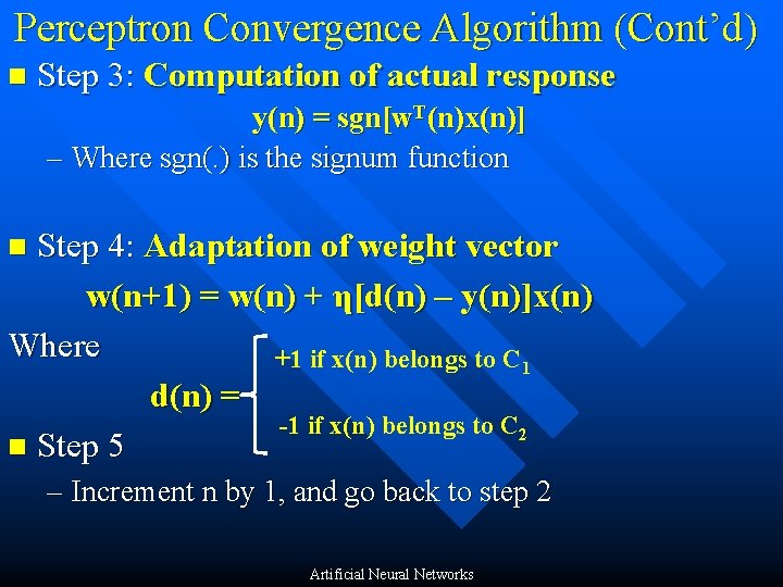
Perceptron Convergence Algorithm n Variables and parameters – x(n) = [+1, x 1(n), …, xp(n)]; w(n) = [b(n), w 1(n), …, wp(n)] – y(n) = actual response (output); d(n) = desired response – η = learning rate, a positive number less than 1 n Step 1: Initialization – Set w(0) = 0, then do the following for n = 1, 2, 3, … n Step 2: Activation – Activate the perceptron by applying input vector x(n) and desired output d(n) Artificial Neural Networks

Perceptron Convergence Algorithm (Cont’d) n Step 3: Computation of actual response y(n) = sgn[w. T(n)x(n)] – Where sgn(. ) is the signum function Step 4: Adaptation of weight vector w(n+1) = w(n) + η[d(n) – y(n)]x(n) Where +1 if x(n) belongs to C 1 d(n) = -1 if x(n) belongs to C 2 n Step 5 n – Increment n by 1, and go back to step 2 Artificial Neural Networks

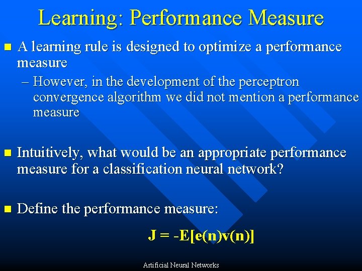
Learning: Performance Measure n A learning rule is designed to optimize a performance measure – However, in the development of the perceptron convergence algorithm we did not mention a performance measure n Intuitively, what would be an appropriate performance measure for a classification neural network? n Define the performance measure: J = -E[e(n)v(n)] Artificial Neural Networks

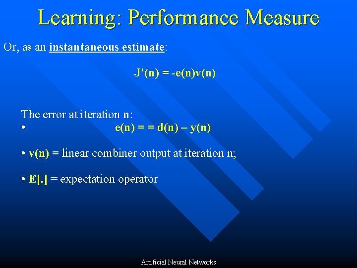
Learning: Performance Measure Or, as an instantaneous estimate: J’(n) = -e(n)v(n) The error at iteration n: • e(n) = = d(n) – y(n) • v(n) = linear combiner output at iteration n; • E[. ] = expectation operator Artificial Neural Networks

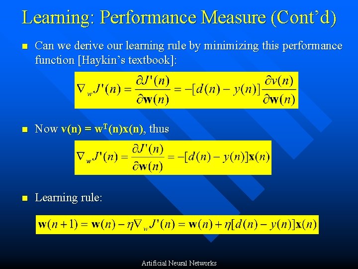
Learning: Performance Measure (Cont’d) n Can we derive our learning rule by minimizing this performance function [Haykin’s textbook]: n Now v(n) = w. T(n)x(n), thus n Learning rule: Artificial Neural Networks

Presentation of Training Examples n Presenting all training examples once to the ANN is called an epoch. n In incremental stochastic gradient descent training examples can be presented in: – Fixed order (1, 2, 3…, M) – Randomly permutated order (5, 2, 7, …, 3) – Completely random (4, 1, 7, 1, 5, 4, ……) Artificial Neural Networks

Concluding Remarks A single layer perceptron can perform pattern classification only on linearly separable patterns, regardless of the type of nonlinearity (hard limiter, sigmoidal) n Papert and Minsky in 1969 elucidated limitations of Rosenblatt’s single layer perceptron (e. g. requirement of linear separability, inability to solve XOR problem) and cast doubt on the viability of neural networks n However, multilayer perceptron and the backpropagation algorithm overcomes many of the shortcomings of the single layer perceptron n Artificial Neural Networks

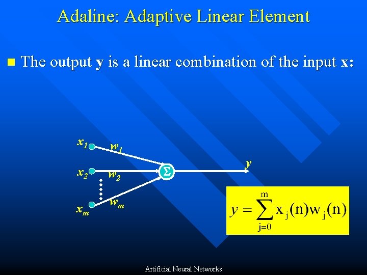
Adaline: Adaptive Linear Element n The output y is a linear combination of the input x: x 1 x 2 xm w 1 w 2 wm Artificial Neural Networks y

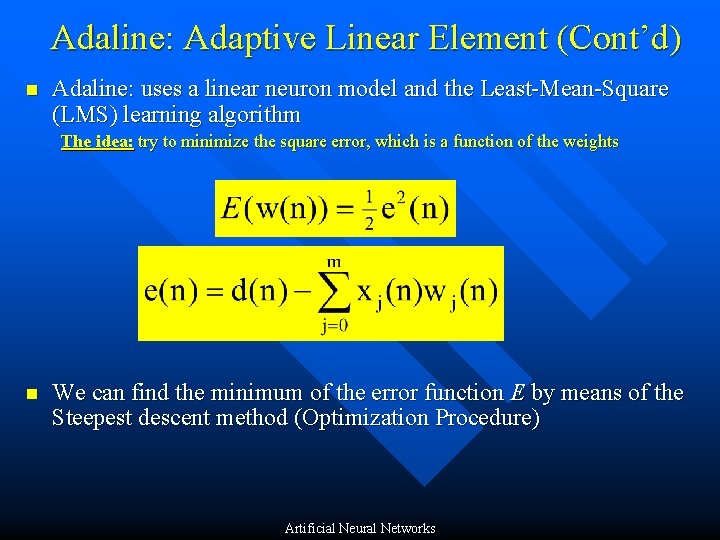
Adaline: Adaptive Linear Element (Cont’d) n Adaline: uses a linear neuron model and the Least-Mean-Square (LMS) learning algorithm The idea: try to minimize the square error, which is a function of the weights n We can find the minimum of the error function E by means of the Steepest descent method (Optimization Procedure) Artificial Neural Networks

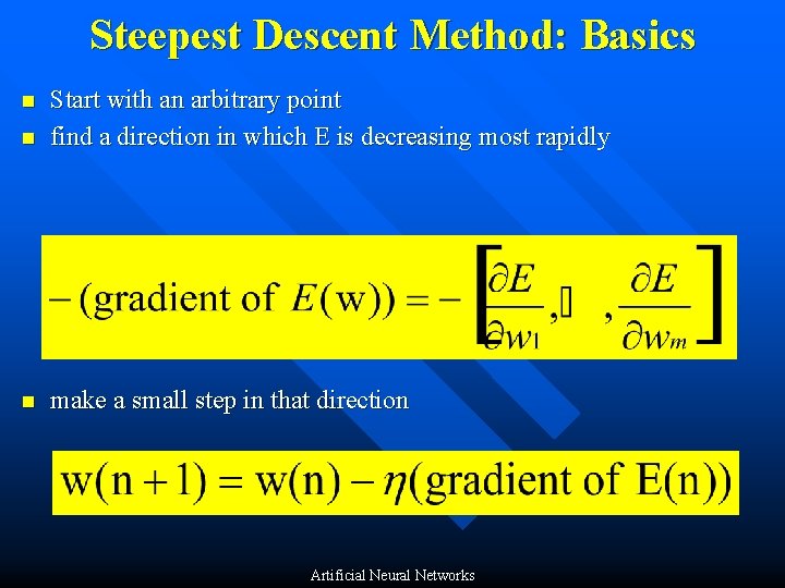
Steepest Descent Method: Basics n Start with an arbitrary point find a direction in which E is decreasing most rapidly n make a small step in that direction n Artificial Neural Networks

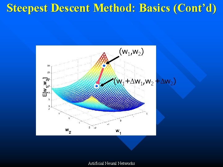
Steepest Descent Method: Basics (Cont’d) (w 1, w 2) (w 1+ w 1, w 2 + w 2) Artificial Neural Networks

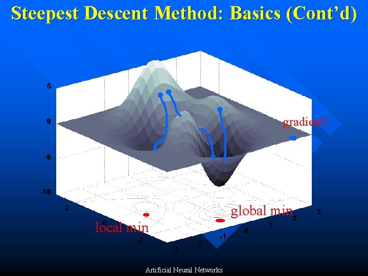
Steepest Descent Method: Basics (Cont’d) gradient? global min local min Artificial Neural Networks

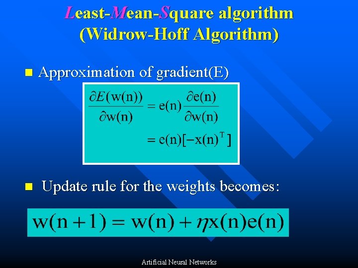
Least-Mean-Square algorithm (Widrow-Hoff Algorithm) n n Approximation of gradient(E) Update rule for the weights becomes: Artificial Neural Networks

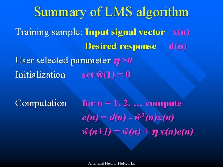
Summary of LMS algorithm Training sample: Input signal vector x(n) Desired response d(n) User selected parameter >0 Initialization set ŵ(1) = 0 Computation for n = 1, 2, … compute e(n) = d(n) - ŵT(n)x(n) ŵ(n+1) = ŵ(n) + x(n)e(n) Artificial Neural Networks

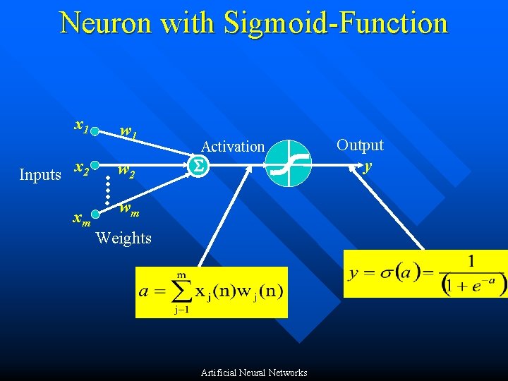
Neuron with Sigmoid-Function x 1 Inputs x 2 xm w 1 w 2 Activation wm Weights Artificial Neural Networks Output y

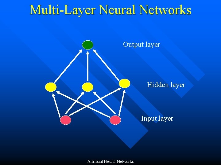
Multi-Layer Neural Networks Output layer Hidden layer Input layer Artificial Neural Networks

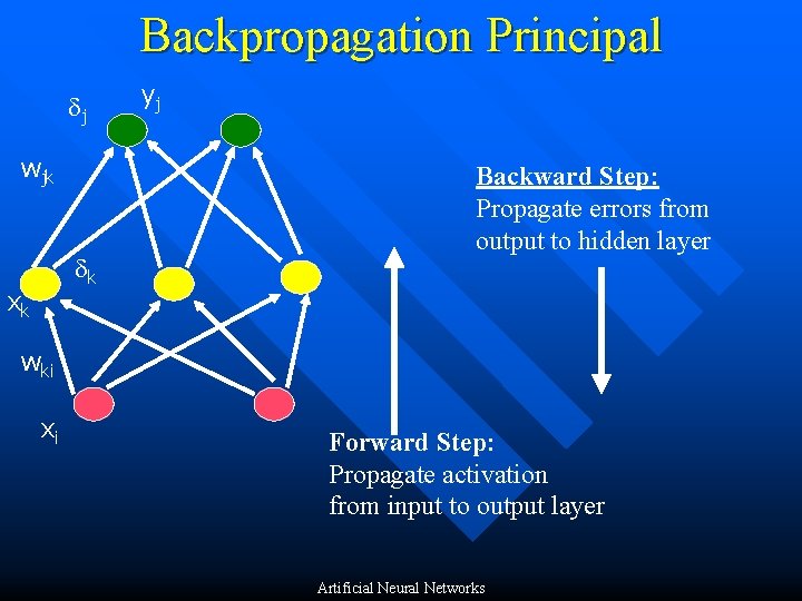
Backpropagation Principal j wjk k xk yj Backward Step: Propagate errors from output to hidden layer wki xi Forward Step: Propagate activation from input to output layer Artificial Neural Networks

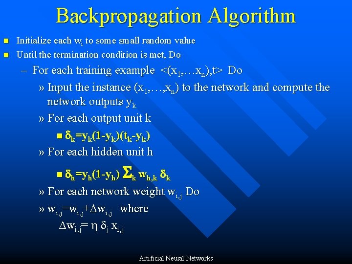
Backpropagation Algorithm n n Initialize each wi to some small random value Until the termination condition is met, Do – For each training example <(x 1, …xn), t> Do » Input the instance (x 1, …, xn) to the network and compute the network outputs yk » For each output unit k n k=yk(1 -yk)(tk-yk) » For each hidden unit h n h=yh(1 -yh) k wh, k k » For each network weight wi, j Do » wi, j=wi, j+ wi, j where wi, j= j xi, j Artificial Neural Networks

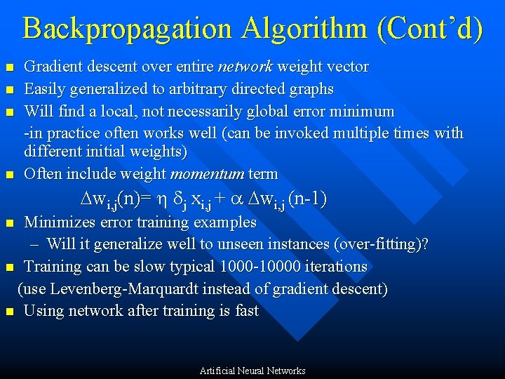
Backpropagation Algorithm (Cont’d) n n Gradient descent over entire network weight vector Easily generalized to arbitrary directed graphs Will find a local, not necessarily global error minimum -in practice often works well (can be invoked multiple times with different initial weights) Often include weight momentum term wi, j(n)= j xi, j + wi, j (n-1) Minimizes error training examples – Will it generalize well to unseen instances (over-fitting)? n Training can be slow typical 1000 -10000 iterations (use Levenberg-Marquardt instead of gradient descent) n Using network after training is fast n Artificial Neural Networks

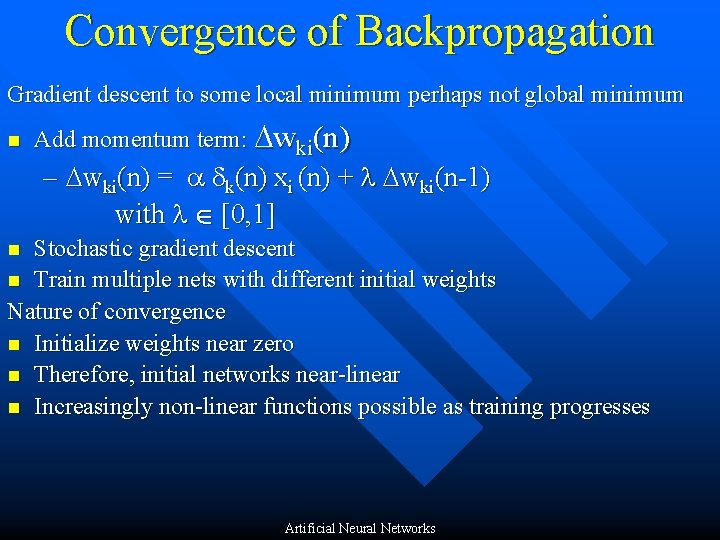
Convergence of Backpropagation Gradient descent to some local minimum perhaps not global minimum n Add momentum term: wki(n) – wki(n) = k(n) xi (n) + l wki(n-1) with l [0, 1] Stochastic gradient descent n Train multiple nets with different initial weights Nature of convergence n Initialize weights near zero n Therefore, initial networks near-linear n Increasingly non-linear functions possible as training progresses n Artificial Neural Networks

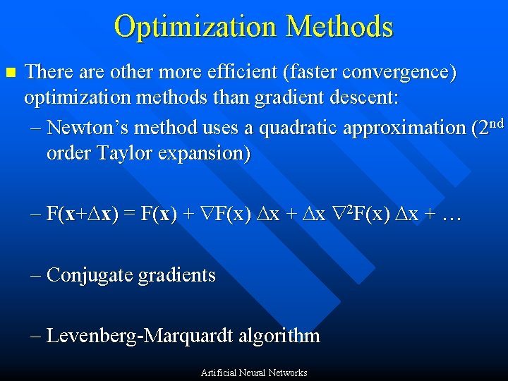
Optimization Methods n There are other more efficient (faster convergence) optimization methods than gradient descent: – Newton’s method uses a quadratic approximation (2 nd order Taylor expansion) – F(x+ x) = F(x) + F(x) x + x 2 F(x) x + … – Conjugate gradients – Levenberg-Marquardt algorithm Artificial Neural Networks

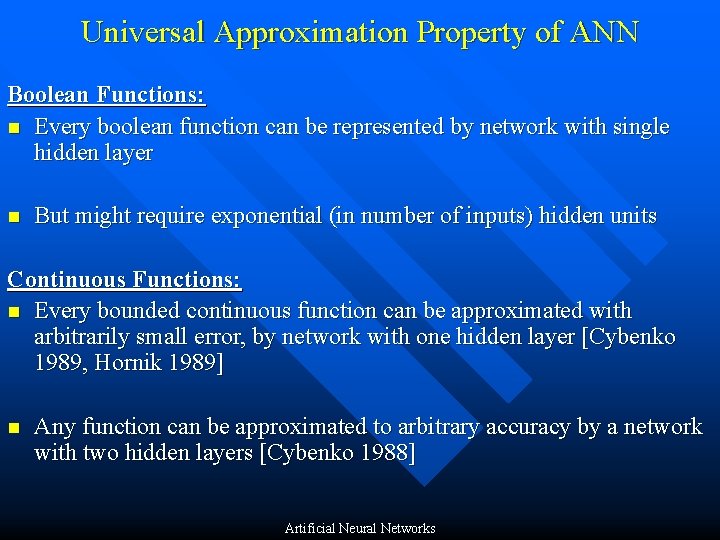
Universal Approximation Property of ANN Boolean Functions: n Every boolean function can be represented by network with single hidden layer n But might require exponential (in number of inputs) hidden units Continuous Functions: n Every bounded continuous function can be approximated with arbitrarily small error, by network with one hidden layer [Cybenko 1989, Hornik 1989] n Any function can be approximated to arbitrary accuracy by a network with two hidden layers [Cybenko 1988] Artificial Neural Networks

Using Weight Derivatives n How often to update – after each training case? – after a full sweep through the training data? n How much to update – Use a fixed learning rate? – Adapt the learning rate? – Add momentum? – Don’t use steepest descent? Artificial Neural Networks

What Next? n Bias Effect n Batch vs. Continuous Learning n Variable Learning Rate (Update Rule? ) n Effect of Neurons/Layer n Effect of Hidden Layers Artificial Neural Networks