Mesh Net Mesh Neural Network for 3 D

Mesh. Net: Mesh Neural Network for 3 D Shape Representation Yutong Feng, Yifan Feng, Haoxuan You, Xibin Zhao , Yue Gao BNRist, KLISS, School of Software, Tsinghua University, China. 2 School of Information Science and Engineering, Xiamen University {feng-yt 15, zxb, gaoyue}@tsinghua. edu. cn, {evanfeng 97, haoxuanyou}@gmail. com

Why mesh Mesh data shows stronger ability to describe 3 D shapes comparing with other popular types of data. • Volumetric grid and multi-view avoid the irregularity of the native data but lose natural information. • Point cloud has ambiguity caused by random sampling and the ambiguity is more obvious with fewer amount of points. However, mesh data is also more irregular and complex for the multiple compositions and varying numbers of elements.

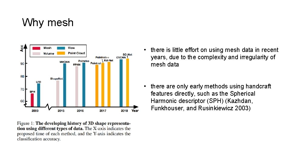
Why mesh • there is little effort on using mesh data in recent years, due to the complexity and irregularity of mesh data • there are only early methods using handcraft features directly, such as the Spherical Harmonic descriptor (SPH) (Kazhdan, Funkhouser, and Rusinkiewicz 2003)

Design ideas l Regard face as the unit. • simplify the data organization • make the connection relationship regular and easy to use • Help to solve the disorder problem l Split feature of face. • for point，need to know “where you are” • for face， want to know “what you look like”

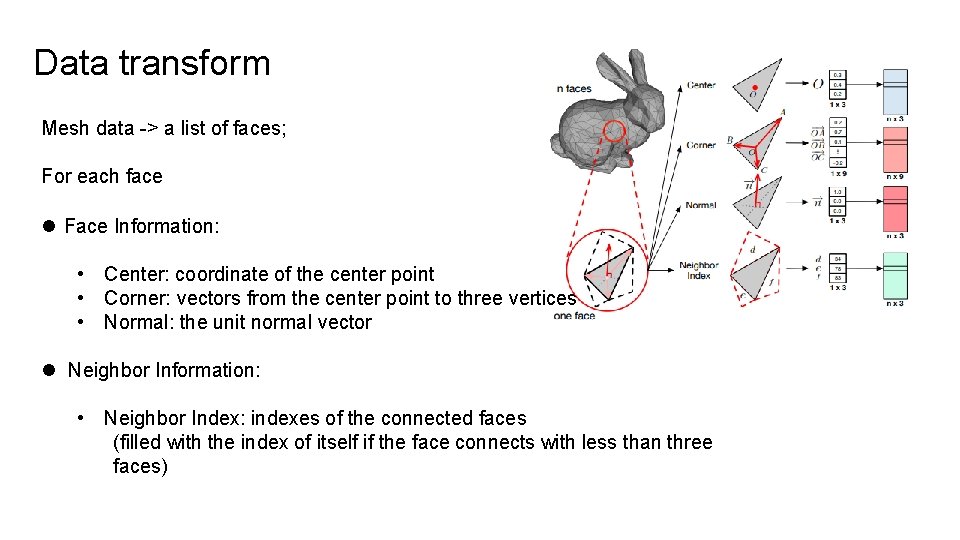
Data transform Mesh data -> a list of faces; For each face l Face Information: • Center: coordinate of the center point • Corner: vectors from the center point to three vertices • Normal: the unit normal vector l Neighbor Information: • Neighbor Index: indexes of the connected faces (filled with the index of itself if the face connects with less than three faces)

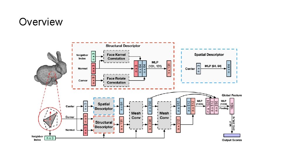
Overview

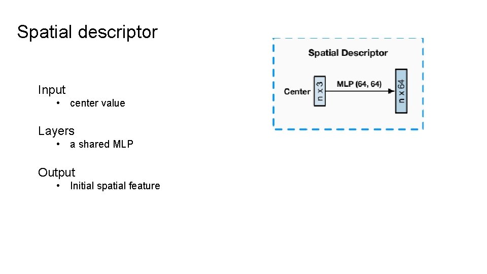
Spatial descriptor Input • center value Layers • a shared MLP Output • Initial spatial feature

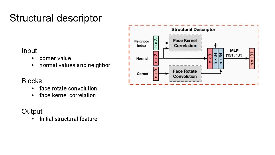
Structural descriptor Input • corner value • normal values and neighbor Blocks • face rotate convolution • face kernel correlation Output • Initial structural feature

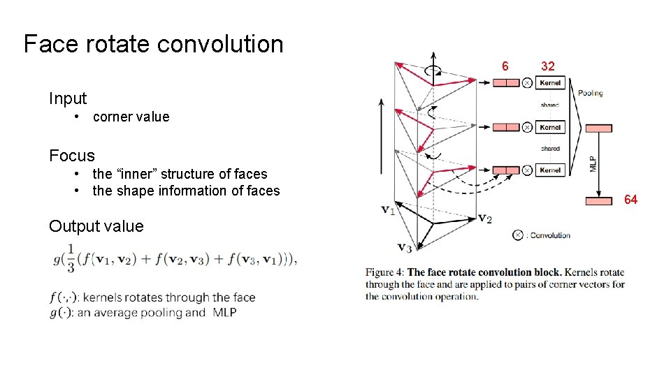
Face rotate convolution 6 32 Input • corner value Focus • the “inner” structure of faces • the shape information of faces Output value 64

Face kernel correlation Input • normal values • neighbors Focus • the “outer” structure of faces • the environments where faces locate

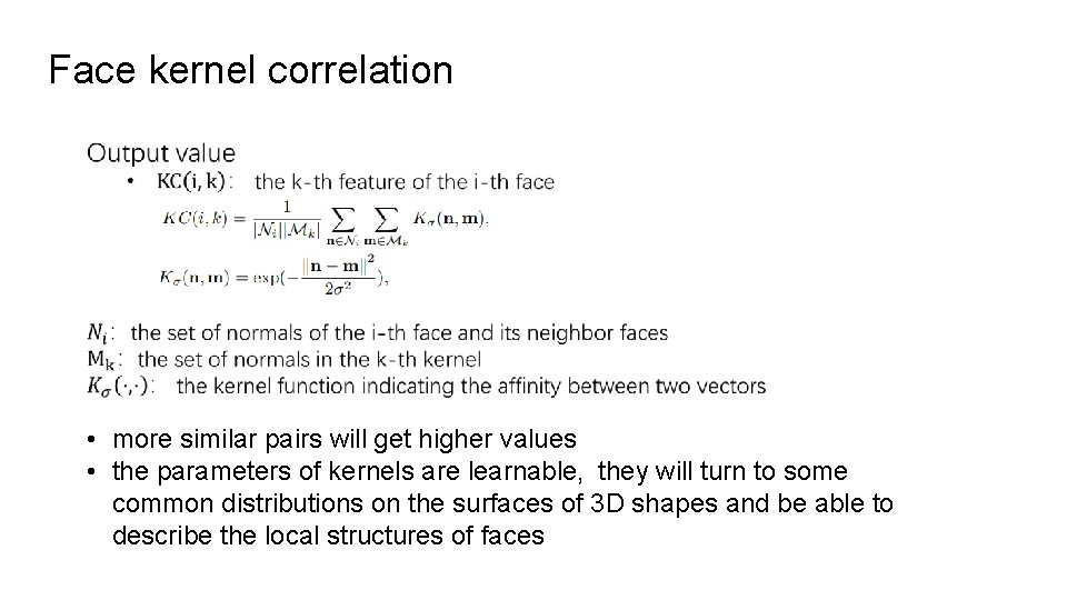
Face kernel correlation • more similar pairs will get higher values • the parameters of kernels are learnable, they will turn to some common distributions on the surfaces of 3 D shapes and be able to describe the local structures of faces

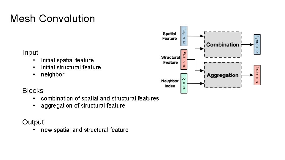
Mesh Convolution Input • Initial spatial feature • Initial structural feature • neighbor Blocks • combination of spatial and structural features • aggregation of structural feature Output • new spatial and structural feature

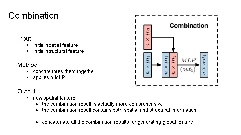
Combination Input • Initial spatial feature • Initial structural feature Method • concatenates them together • applies a MLP Output • new spatial feature Ø the combination result is actually more comprehensive Ø the combination result contains both spatial and structural information Ø concatenate all the combination results for generating global feature

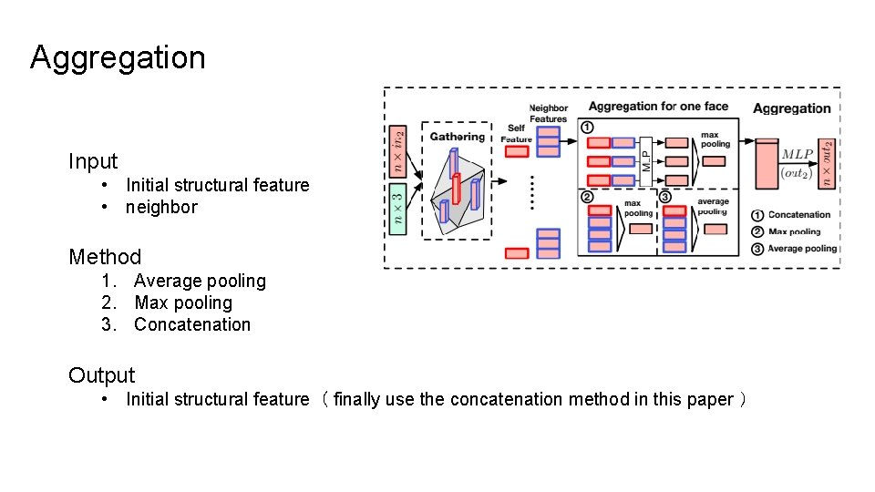
Aggregation Input • Initial structural feature • neighbor Method 1. Average pooling 2. Max pooling 3. Concatenation Output • Initial structural feature（ finally use the concatenation method in this paper ）

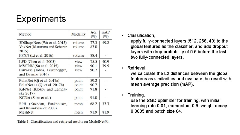
Experiments • Classification, apply fully-connected layers (512, 256, 40) to the global features as the classifier, and add dropout layers with drop probability of 0. 5 before the last two fully-connected layers. • Retrieval, we calculate the L 2 distances between the global features as similarities and evaluate the result with mean average precision (m. AP). • Training， use the SGD optimizer for training, with initial learning rate 0. 01, momentum 0. 9, weight decay 0. 0005 and batch size 64.

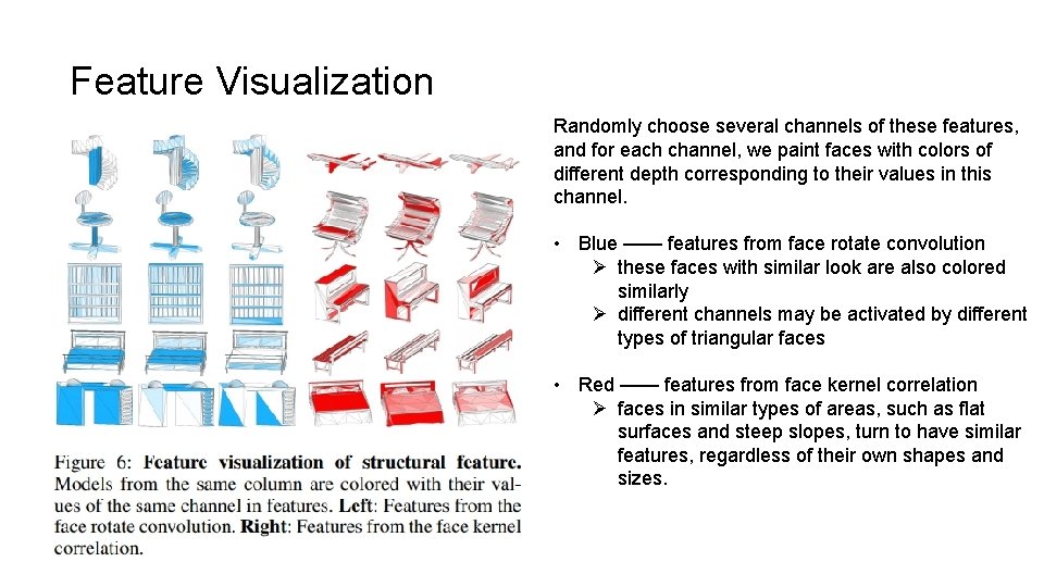
Feature Visualization Randomly choose several channels of these features, and for each channel, we paint faces with colors of different depth corresponding to their values in this channel. • Blue —— features from face rotate convolution Ø these faces with similar look are also colored similarly Ø different channels may be activated by different types of triangular faces • Red —— features from face kernel correlation Ø faces in similar types of areas, such as flat surfaces and steep slopes, turn to have similar features, regardless of their own shapes and sizes.