Neural Network Part 1 Multiple Layer Neural Networks

Neural Network Part 1: Multiple Layer Neural Networks Yingyu Liang Computer Sciences 760 Fall 2017 http: //pages. cs. wisc. edu/~yliang/cs 760/ Some of the slides in these lectures have been adapted/borrowed from materials developed by Mark Craven, David Page, Jude Shavlik, Tom Mitchell, Nina Balcan, Matt Gormley, Elad Hazan, Tom Dietterich, and Pedro Domingos.

Goals for the lecture you should understand the following concepts • perceptrons • the perceptron training rule • linear separability • multilayer neural networks • stochastic gradient descent • backpropagation 2

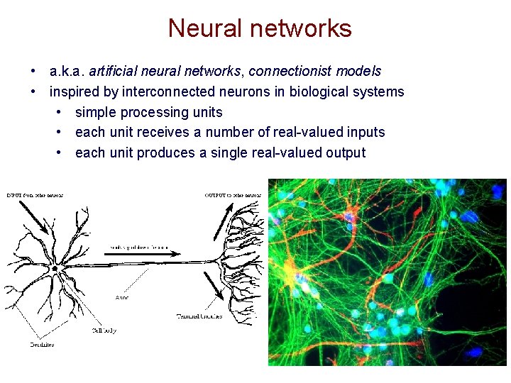
Neural networks • a. k. a. artificial neural networks, connectionist models • inspired by interconnected neurons in biological systems • simple processing units • each unit receives a number of real-valued inputs • each unit produces a single real-valued output 3

Perceptrons [Mc. Culloch & Pitts, 1943; Rosenblatt, 1959; Widrow & Hoff, 1960] input units: represent given x output unit: represents binary classification 4

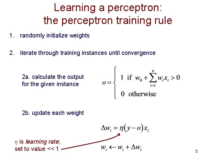
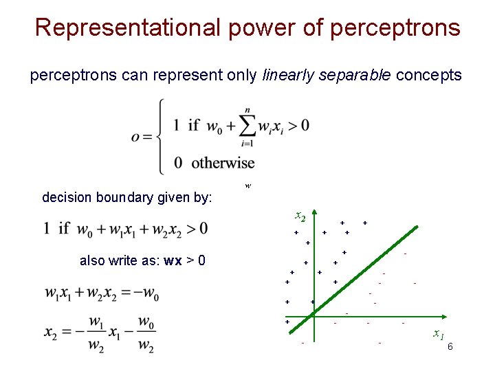
Learning a perceptron: the perceptron training rule 1. randomly initialize weights 2. iterate through training instances until convergence 2 a. calculate the output for the given instance 2 b. update each weight η is learning rate; set to value << 1 5

Representational power of perceptrons can represent only linearly separable concepts decision boundary given by: x 2 + + + also write as: wx > 0 + + - - + + - - - x 1 6

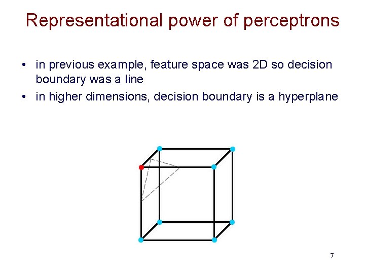
Representational power of perceptrons • in previous example, feature space was 2 D so decision boundary was a line • in higher dimensions, decision boundary is a hyperplane 7

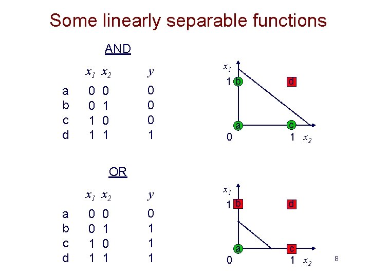
Some linearly separable functions AND a b c d x 1 x 2 y 0 0 1 1 0 0 0 1 0 1 x 1 1 b a 0 d c 1 x 2 OR a b c d x 1 x 2 y 0 0 1 1 1 0 1 x 1 1 b a 0 d c 1 x 2 8

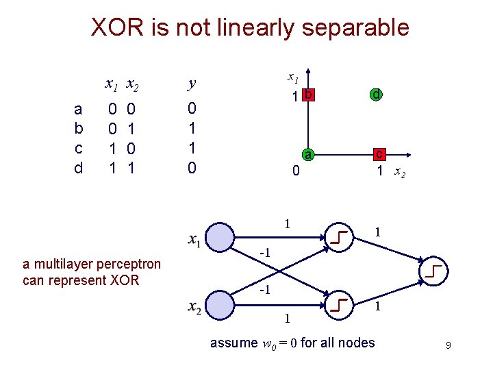
XOR is not linearly separable a b c d x 1 x 2 y 0 0 1 1 0 0 1 x 1 1 b c 1 x 2 a 0 1 a multilayer perceptron can represent XOR d 1 -1 -1 1 1 assume w 0 = 0 for all nodes 9

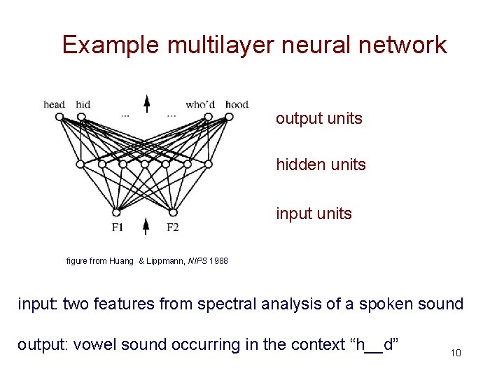
Example multilayer neural network output units hidden units input units figure from Huang & Lippmann, NIPS 1988 input: two features from spectral analysis of a spoken sound output: vowel sound occurring in the context “h__d” 10

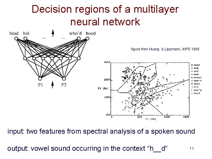
Decision regions of a multilayer neural network figure from Huang & Lippmann, NIPS 1988 input: two features from spectral analysis of a spoken sound output: vowel sound occurring in the context “h__d” 11

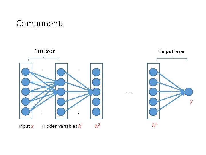
Components • Representations: • Input • Hidden variables • Layers/weights: • Hidden layers • Output layer

Components First layer Output layer … … …

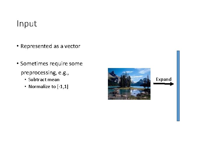
Input • Represented as a vector • Sometimes require some preprocessing, e. g. , • Subtract mean • Normalize to [-1, 1] Expand

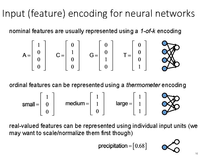
Input (feature) encoding for neural networks nominal features are usually represented using a 1 -of-k encoding ordinal features can be represented using a thermometer encoding real-valued features can be represented using individual input units (we may want to scale/normalize them first though) 15

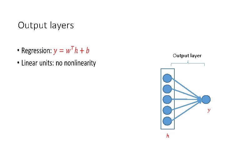
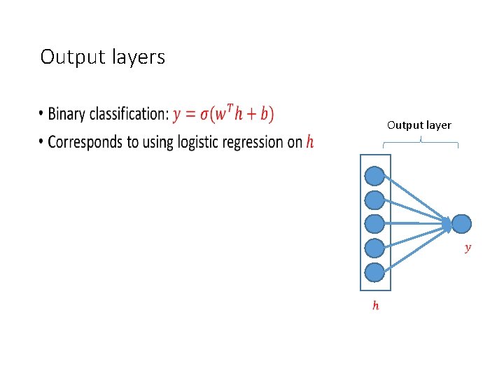
Output layers • Output layer

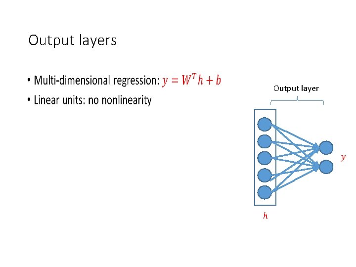
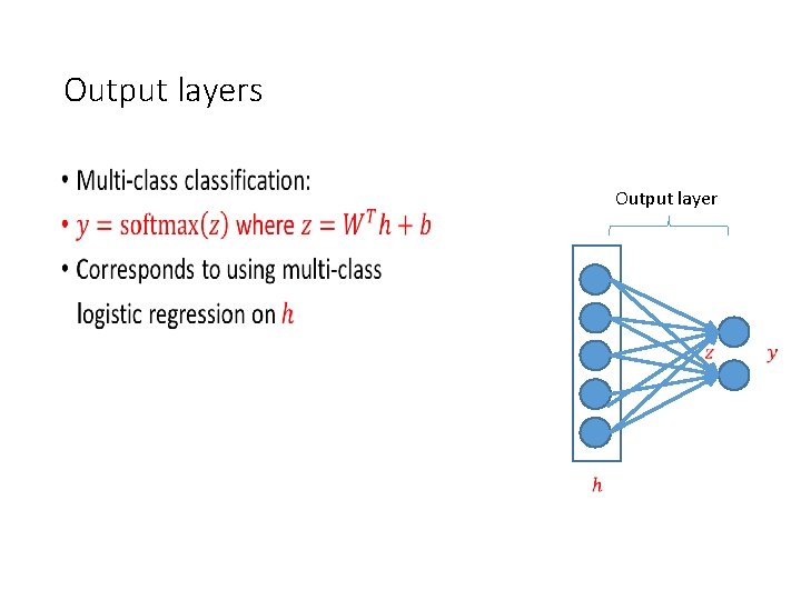
Output layers • Output layer

Output layers • Output layer

Output layers • Output layer

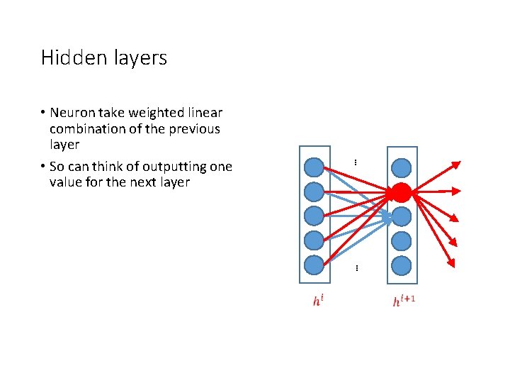
Hidden layers … • Neuron take weighted linear combination of the previous layer • So can think of outputting one value for the next layer …

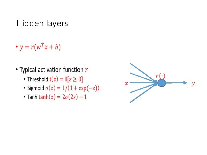
Hidden layers •

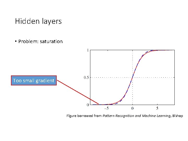
Hidden layers • Problem: saturation Too small gradient Figure borrowed from Pattern Recognition and Machine Learning, Bishop

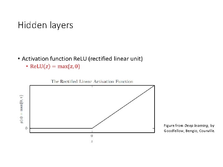
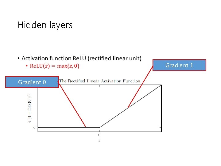
Hidden layers • Figure from Deep learning, by Goodfellow, Bengio, Courville.

Hidden layers • Gradient 0 Gradient 1

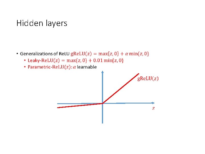
Hidden layers •

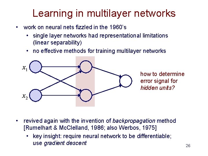
Learning in multilayer networks • work on neural nets fizzled in the 1960’s • single layer networks had representational limitations (linear separability) • no effective methods for training multilayer networks how to determine error signal for hidden units? • revived again with the invention of backpropagation method [Rumelhart & Mc. Clelland, 1986; also Werbos, 1975] • key insight: require neural network to be differentiable; use gradient descent 26

Learning in multilayer networks • learning techniques nowadays • random initialization of the weights • stochastic gradient descent (can add momentum) • regularization techniques • norm constraint • dropout • batch normalization • data augmentation • early stopping • pretraining • …

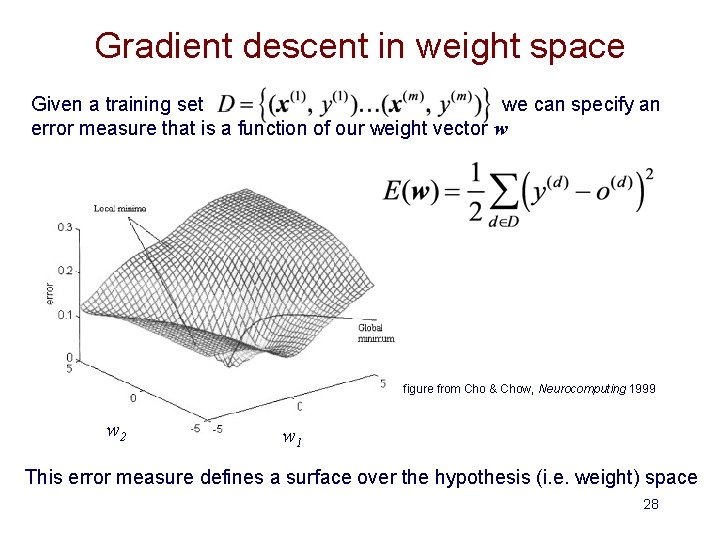
Gradient descent in weight space Given a training set we can specify an error measure that is a function of our weight vector w figure from Cho & Chow, Neurocomputing 1999 w 2 w 1 This error measure defines a surface over the hypothesis (i. e. weight) space 28

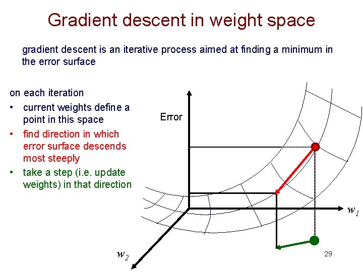
Gradient descent in weight space gradient descent is an iterative process aimed at finding a minimum in the error surface on each iteration • current weights define a point in this space • find direction in which error surface descends most steeply • take a step (i. e. update weights) in that direction Error w 1 w 2 29

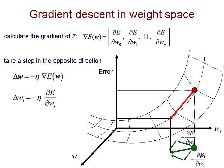
Gradient descent in weight space calculate the gradient of E: take a step in the opposite direction Error w 1 w 2 30

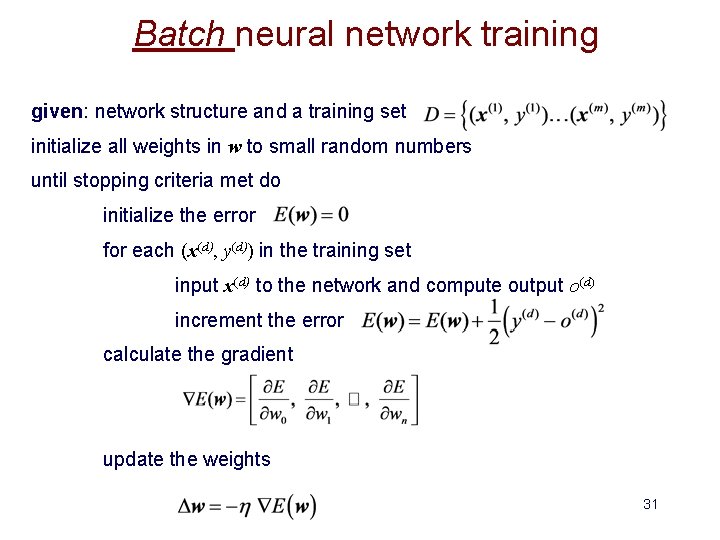
Batch neural network training given: network structure and a training set initialize all weights in w to small random numbers until stopping criteria met do initialize the error for each (x(d), y(d)) in the training set input x(d) to the network and compute output o(d) increment the error calculate the gradient update the weights 31

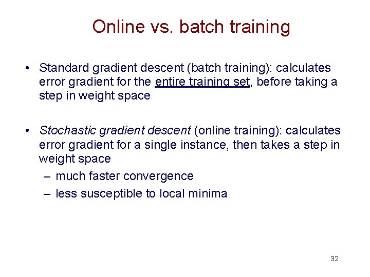
Online vs. batch training • Standard gradient descent (batch training): calculates error gradient for the entire training set, before taking a step in weight space • Stochastic gradient descent (online training): calculates error gradient for a single instance, then takes a step in weight space – much faster convergence – less susceptible to local minima 32

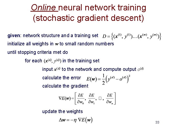
Online neural network training (stochastic gradient descent) given: network structure and a training set initialize all weights in w to small random numbers until stopping criteria met do for each (x(d), y(d)) in the training set input x(d) to the network and compute output o(d) calculate the error calculate the gradient update the weights 33

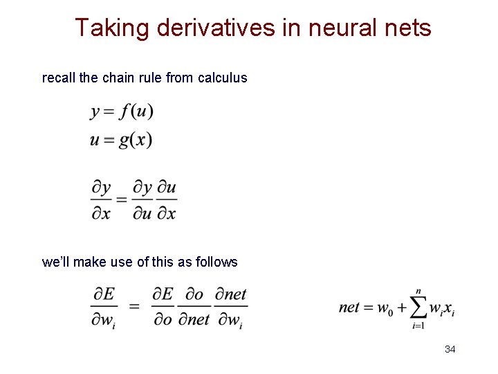
Taking derivatives in neural nets recall the chain rule from calculus we’ll make use of this as follows 34

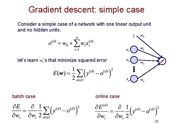
Gradient descent: simple case Consider a simple case of a network with one linear output unit and no hidden units: let’s learn wi’s that minimize squared error batch case online case 35

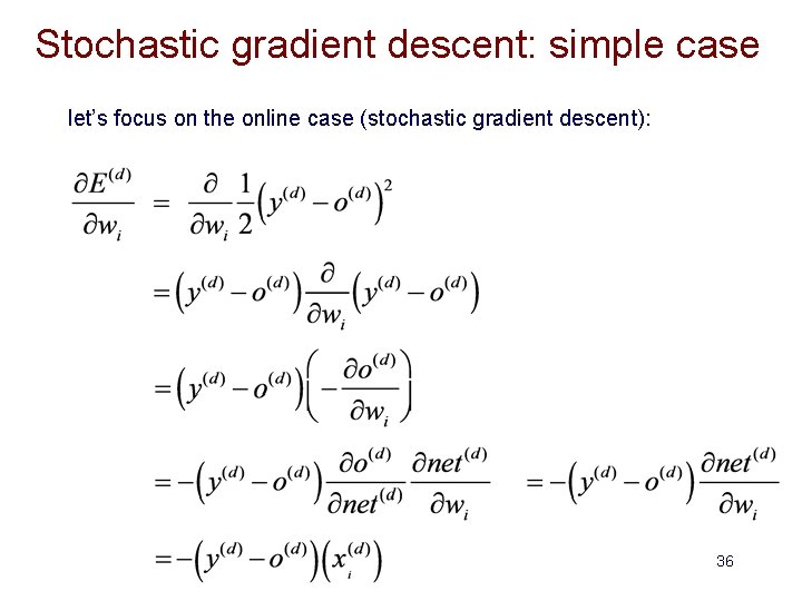
Stochastic gradient descent: simple case let’s focus on the online case (stochastic gradient descent): 36

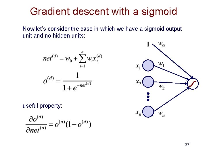
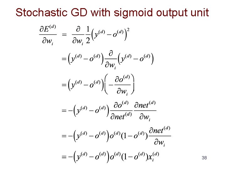
Gradient descent with a sigmoid Now let’s consider the case in which we have a sigmoid output unit and no hidden units: useful property: 37

Stochastic GD with sigmoid output unit 38

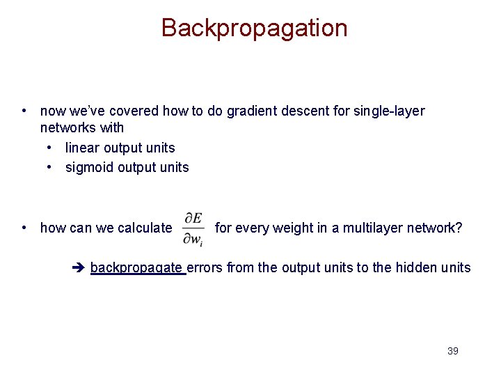
Backpropagation • now we’ve covered how to do gradient descent for single-layer networks with • linear output units • sigmoid output units • how can we calculate for every weight in a multilayer network? backpropagate errors from the output units to the hidden units 39

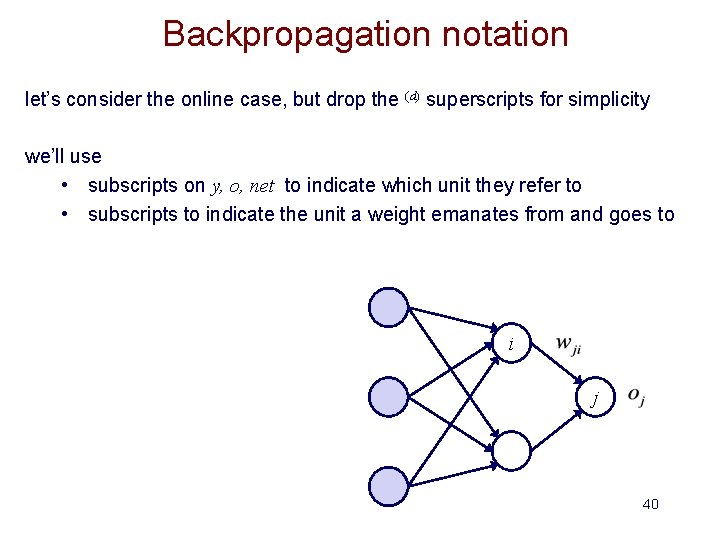
Backpropagation notation let’s consider the online case, but drop the (d) superscripts for simplicity we’ll use • subscripts on y, o, net to indicate which unit they refer to • subscripts to indicate the unit a weight emanates from and goes to i j 40

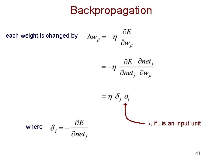
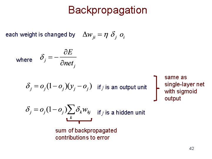
Backpropagation each weight is changed by where xi if i is an input unit 41

Backpropagation each weight is changed by where if j is an output unit same as single-layer net with sigmoid output if j is a hidden unit sum of backpropagated contributions to error 42

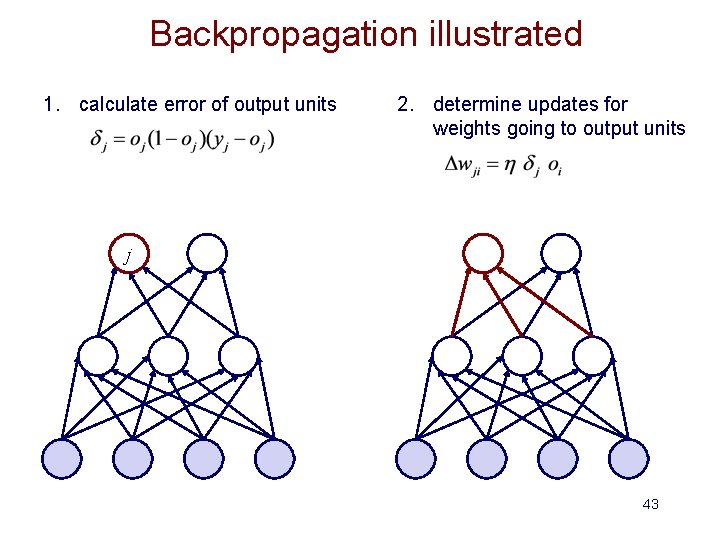
Backpropagation illustrated 1. calculate error of output units 2. determine updates for weights going to output units j 43

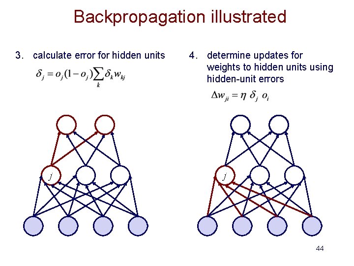
Backpropagation illustrated 3. calculate error for hidden units j 4. determine updates for weights to hidden units using hidden-unit errors j 44