Neural networks 1 Neural networks Neural networks are

Neural networks 1

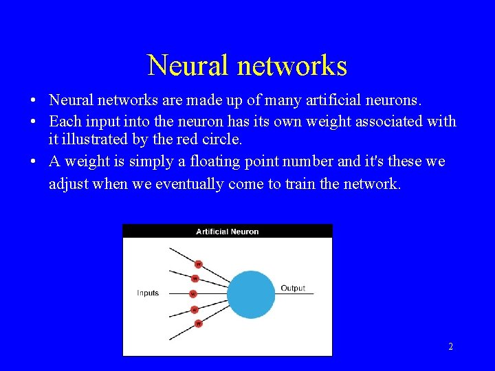
Neural networks • Neural networks are made up of many artificial neurons. • Each input into the neuron has its own weight associated with it illustrated by the red circle. • A weight is simply a floating point number and it's these we adjust when we eventually come to train the network. 2

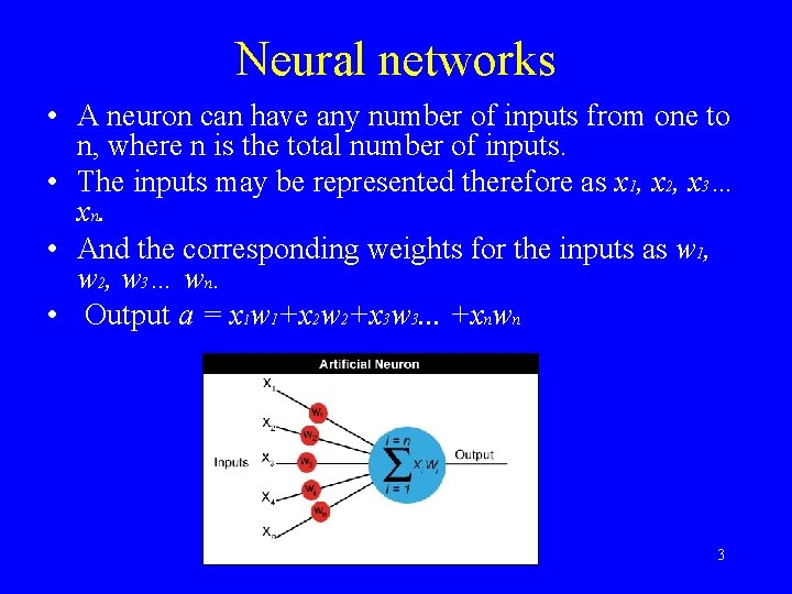
Neural networks • A neuron can have any number of inputs from one to n, where n is the total number of inputs. • The inputs may be represented therefore as x 1, x 2, x 3… xn. • And the corresponding weights for the inputs as w 1, w 2, w 3… wn. • Output a = x 1 w 1+x 2 w 2+x 3 w 3. . . +xnwn 3

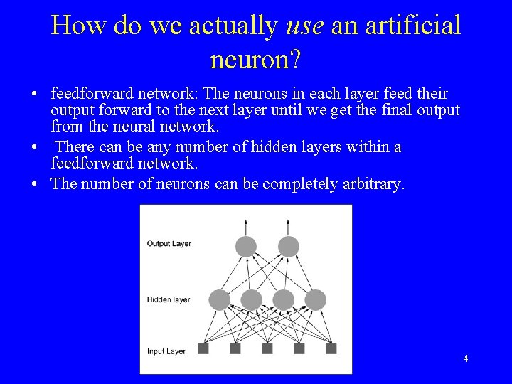
How do we actually use an artificial neuron? • feedforward network: The neurons in each layer feed their output forward to the next layer until we get the final output from the neural network. • There can be any number of hidden layers within a feedforward network. • The number of neurons can be completely arbitrary. 4

Neural Networks by an Example • initialize the neural net with random weights • feed it a series of inputs which represent, in this example, the different panel configurations • For each configuration we check to see what its output is and adjust the weights accordingly. 5

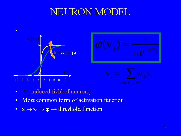
NEURON MODEL • Sigmoidal Function 1 Increasing a -10 -8 -6 -4 -2 2 4 6 8 10 • induced field of neuron j • Most common form of activation function • a threshold functiontiable 6

Multi-Layer Perceptron (MLP) 7

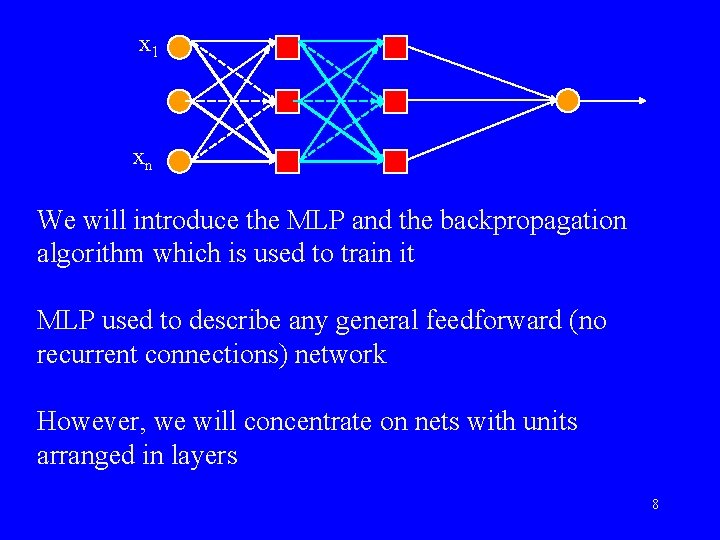
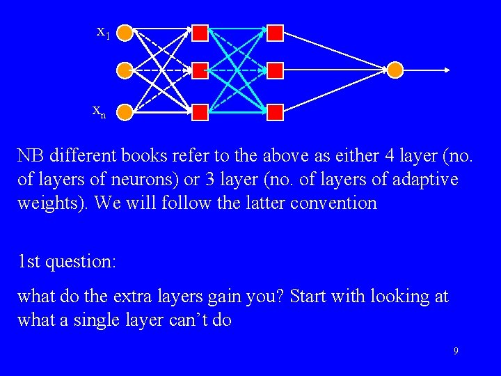
x 1 xn We will introduce the MLP and the backpropagation algorithm which is used to train it MLP used to describe any general feedforward (no recurrent connections) network However, we will concentrate on nets with units arranged in layers 8

x 1 xn NB different books refer to the above as either 4 layer (no. of layers of neurons) or 3 layer (no. of layers of adaptive weights). We will follow the latter convention 1 st question: what do the extra layers gain you? Start with looking at what a single layer can’t do 9

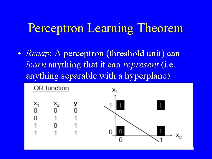
Perceptron Learning Theorem • Recap: A perceptron (threshold unit) can learn anything that it can represent (i. e. anything separable with a hyperplane) 10

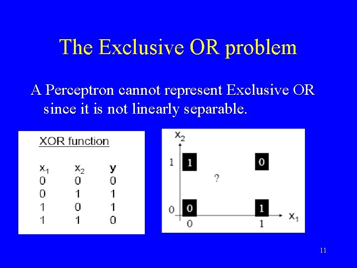
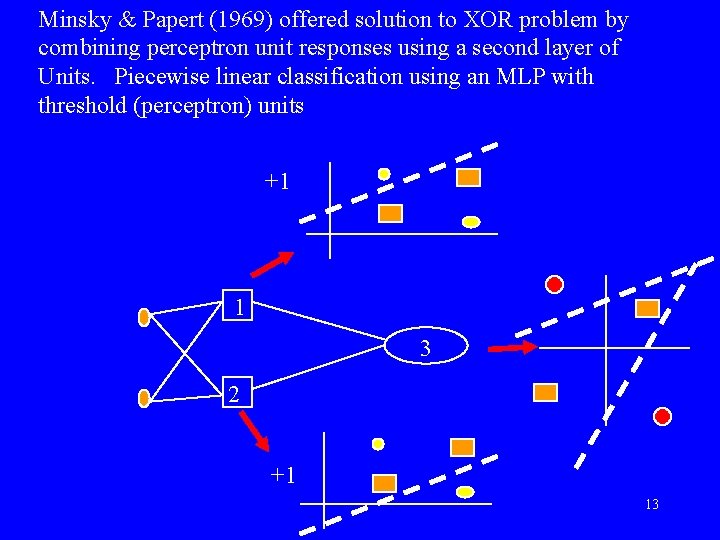
The Exclusive OR problem A Perceptron cannot represent Exclusive OR since it is not linearly separable. 11

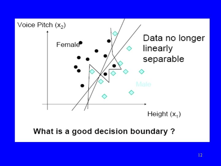
12

Minsky & Papert (1969) offered solution to XOR problem by combining perceptron unit responses using a second layer of Units. Piecewise linear classification using an MLP with threshold (perceptron) units +1 1 3 2 +1 13

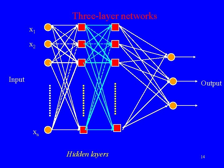
Three-layer networks x 1 x 2 Input Output xn Hidden layers 14

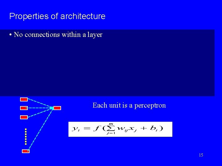
Properties of architecture • No connections within a layer Each unit is a perceptron 15

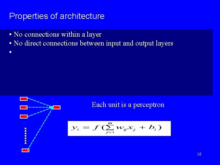
Properties of architecture • No connections within a layer • No direct connections between input and output layers • Each unit is a perceptron 16

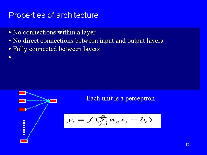
Properties of architecture • No connections within a layer • No direct connections between input and output layers • Fully connected between layers • Each unit is a perceptron 17

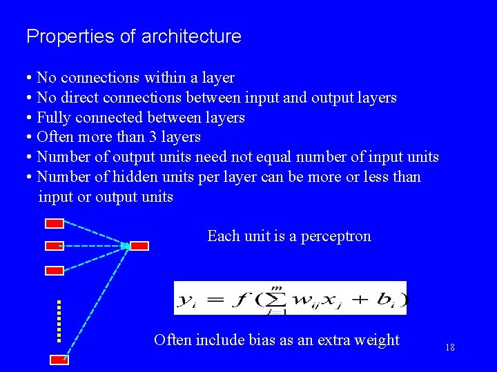
Properties of architecture • No connections within a layer • No direct connections between input and output layers • Fully connected between layers • Often more than 3 layers • Number of output units need not equal number of input units • Number of hidden units per layer can be more or less than input or output units Each unit is a perceptron Often include bias as an extra weight 18

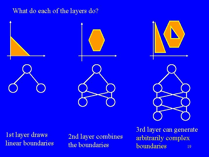
What do each of the layers do? 1 st layer draws linear boundaries 2 nd layer combines the boundaries 3 rd layer can generate arbitrarily complex 19 boundaries

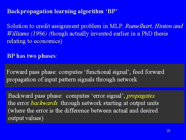
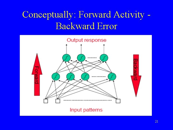
Backpropagation learning algorithm ‘BP’ Solution to credit assignment problem in MLP. Rumelhart, Hinton and Williams (1986) (though actually invented earlier in a Ph. D thesis relating to economics) BP has two phases: Forward pass phase: computes ‘functional signal’, feed forward propagation of input pattern signals through network Backward pass phase: computes ‘error signal’, propagates the error backwards through network starting at output units (where the error is the difference between actual and desired output values) 20

Conceptually: Forward Activity Backward Error 21

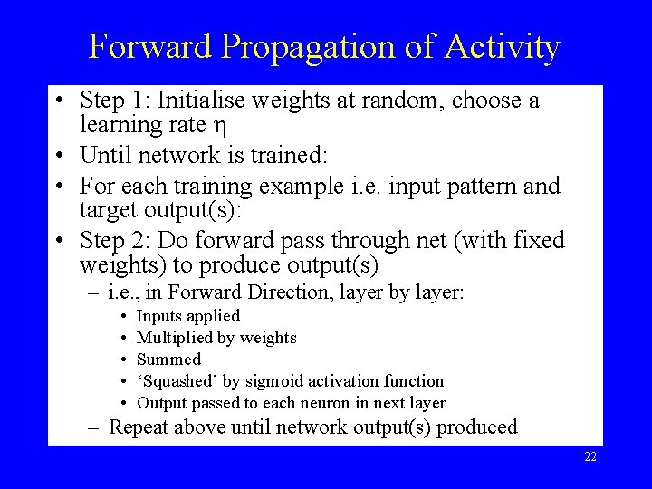
Forward Propagation of Activity • Step 1: Initialise weights at random, choose a learning rate η • Until network is trained: • For each training example i. e. input pattern and target output(s): • Step 2: Do forward pass through net (with fixed weights) to produce output(s) – i. e. , in Forward Direction, layer by layer: • • • Inputs applied Multiplied by weights Summed ‘Squashed’ by sigmoid activation function Output passed to each neuron in next layer – Repeat above until network output(s) produced 22

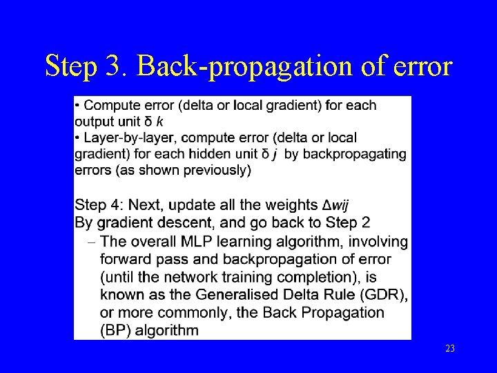
Step 3. Back-propagation of error 23

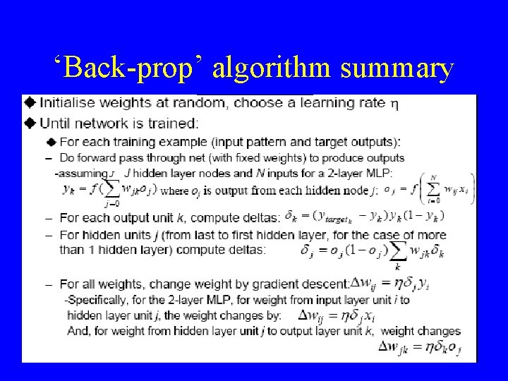
‘Back-prop’ algorithm summary 24

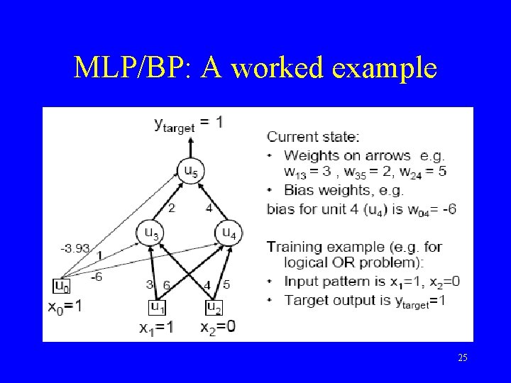
MLP/BP: A worked example 25

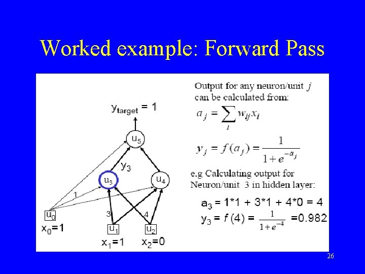
Worked example: Forward Pass 26

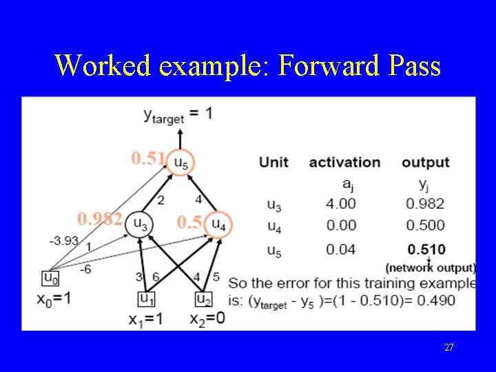
Worked example: Forward Pass 27

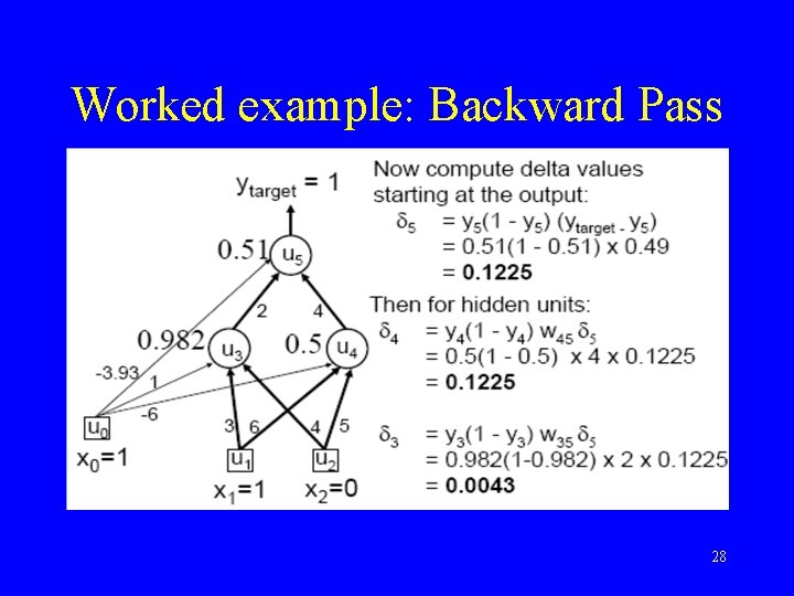
Worked example: Backward Pass 28

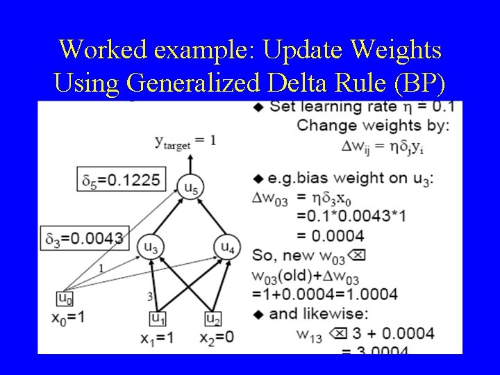
Worked example: Update Weights Using Generalized Delta Rule (BP) 29

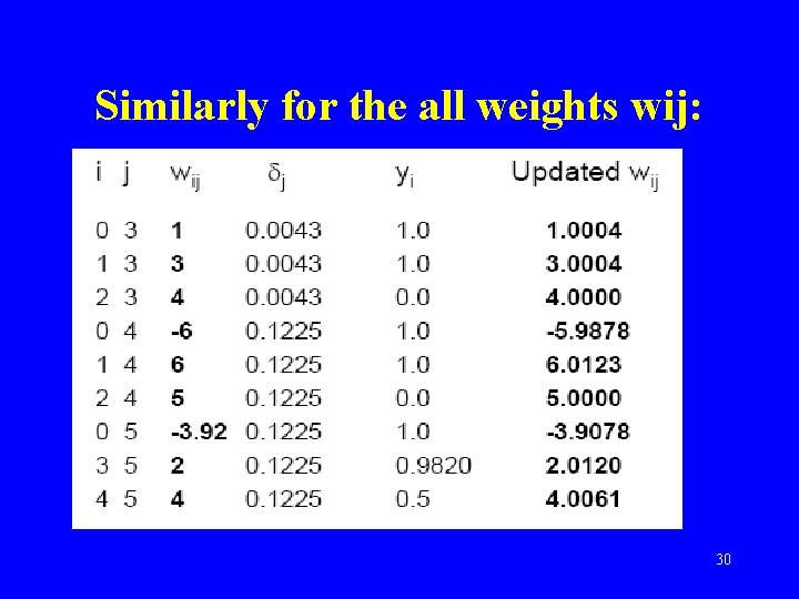
Similarly for the all weights wij: 30

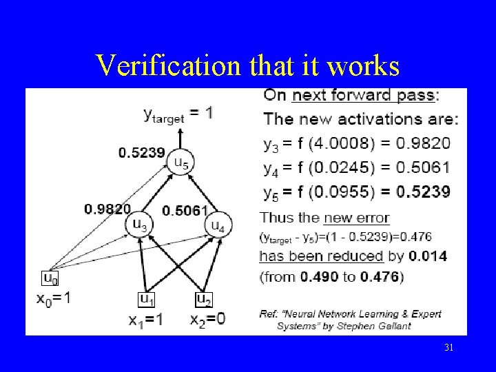
Verification that it works 31

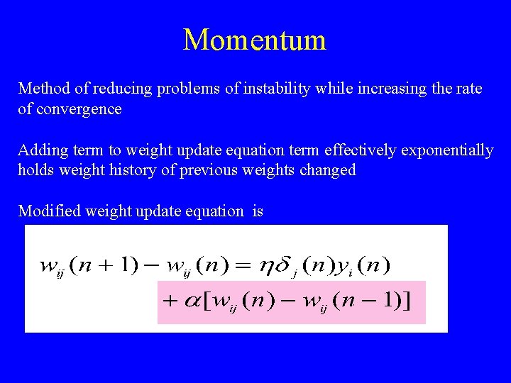
Momentum Method of reducing problems of instability while increasing the rate of convergence Adding term to weight update equation term effectively exponentially holds weight history of previous weights changed Modified weight update equation is

Training • This was a single iteration of back-prop • Training requires many iterations with many training examples or epochs (one epoch is entire presentation of complete training set) • It can be slow ! • Note that computation in MLP is local (with respect to each neuron) • Parallel computation implementation is also possible 33

a is momentum constant and controls how much notice is taken of recent history Effect of momentum term • If weight changes tend to have same sign momentum terms increases and gradient decrease speed up convergence on shallow gradient • If weight changes tend have opposing signs momentum term decreases and gradient descent slows to reduce oscillations (stablizes) • Can help escape being trapped in local minima

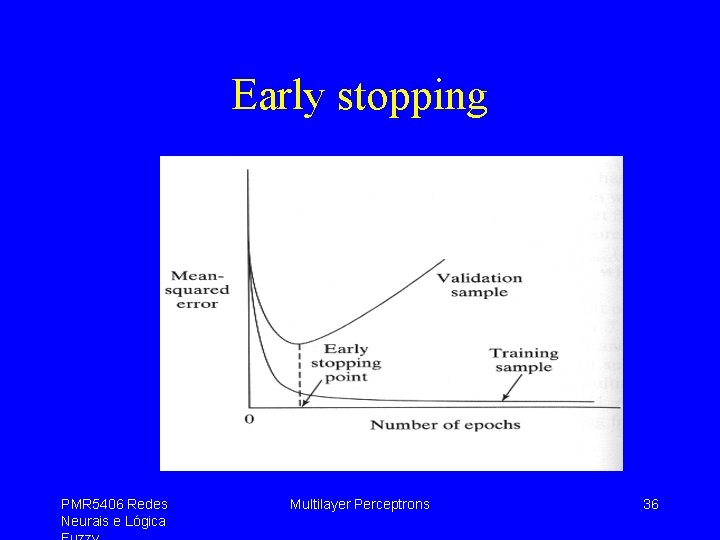
Stopping criteria • Sensible stopping criteria: – Average squared error change: Back-prop is considered to have converged when the absolute rate of change in the average squared error per epoch is sufficiently small (in the range [0. 1, 0. 01]). – Generalization based criterion: After each epoch the NN is tested for generalization. If the generalization performance is adequate then stop. 35

Early stopping PMR 5406 Redes Neurais e Lógica Multilayer Perceptrons 36

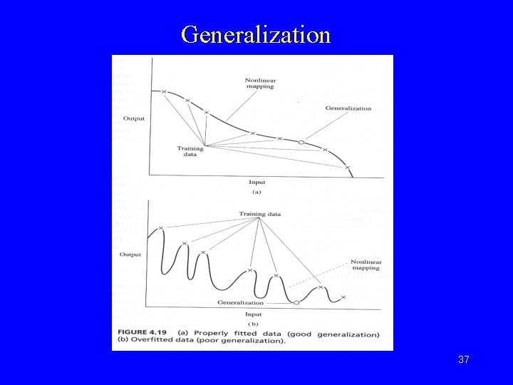
Generalization 37

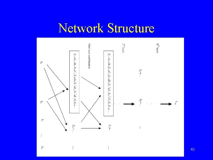
GMDH • Introduced by Ivakhnenko in 1966 • Group Method of Data Handling is the realization of inductive approach for mathematical modeling of complex systems. • A data-driven modeling method that approximates a given variable y (output) as a function of a set of input variables 38

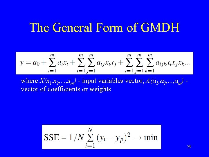
The General Form of GMDH where X(x 1, x 2, . . . , xm) - input variables vector; A(a 1, a 2, . . . , am) - vector of coefficients or weights 39

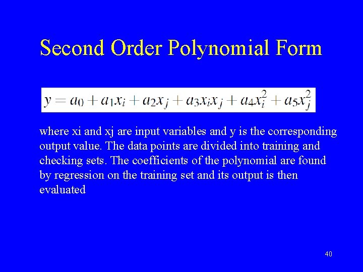
Second Order Polynomial Form where xi and xj are input variables and y is the corresponding output value. The data points are divided into training and checking sets. The coefficients of the polynomial are found by regression on the training set and its output is then evaluated 40

Network Structure 41

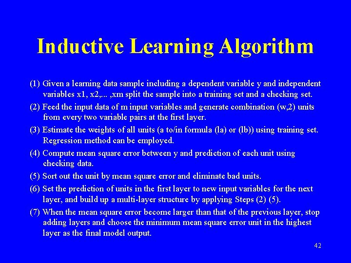
Inductive Learning Algorithm (1) Given a learning data sample including a dependent variable y and independent variables x 1, x 2, . . . , xm split the sample into a training set and a checking set. (2) Feed the input data of m input variables and generate combination (w, 2) units from every two variable pairs at the first layer. (3) Estimate the weights of all units (a to/in formula (la) or (lb)) using training set. Regression method can be employed. (4) Compute mean square error between y and prediction of each unit using checking data. (5) Sort out the unit by mean square error and eliminate bad units. (6) Set the prediction of units in the first layer to new input variables for the next layer, and build up a multi-layer structure by applying Steps (2) (5). (7) When the mean square error become larger than that of the previous layer, stop adding layers and choose the minimum mean square error unit in the highest layer as the final model output. 42

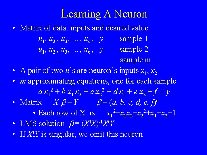
Learning A Neuron • Matrix of data: inputs and desired value u 1, u 2 , u 3, …, un , y sample 1 u 1, u 2 , u 3, …, un , y sample 2 …. sample m • A pair of two u’s are neuron’s inputs x 1, x 2 • m approximating equations, one for each sample a x 12 + b x 1 x 2 + c x 22 + d x 1 + e x 2 + f = y • Matrix X = Y = (a, b, c, d, e, f)t • Each row of X is x 12+x 1 x 2+x 22+x 1+x 2+1 • LMS solution = (Xt. X)-1 Xt. Y • If Xt. X is singular, we omit this neuron

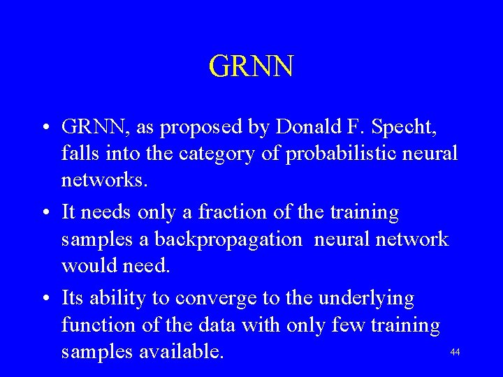
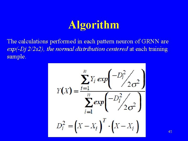
GRNN • GRNN, as proposed by Donald F. Specht, falls into the category of probabilistic neural networks. • It needs only a fraction of the training samples a backpropagation neural network would need. • Its ability to converge to the underlying function of the data with only few training 44 samples available.

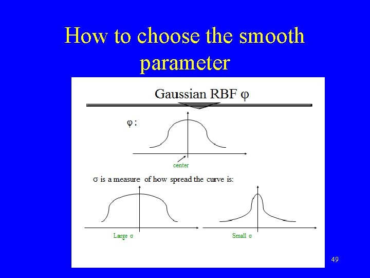
Algorithm The calculations performed in each pattern neuron of GRNN are exp(-Dj 2/2 s 2), the normal distribution centered at each training sample. 45

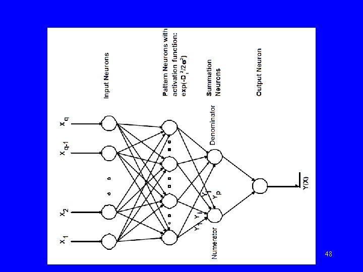
Structures of GRNN • Input layer — There is one neuron in the input layer for each predictor variable. The input neurons then feed the values to each of the neurons in the hidden layer. • Hidden layer — This layer has one neuron for each case in the training data set. The neuron stores the values of the predictor variables for the case along with the target value. When presented with the x vector of input values from the input layer, a hidden neuron computes the Euclidean distance of the test case from the neuron’s center point and then applies the RBF kernel function using the sigma value(s). The resulting value is passed to the neurons in the pattern layer. 46

• Pattern layer / Summation layer — There are only two neurons in the pattern layer. One neuron is the denominator summation unit the other is the numerator summation unit. The denominator summation unit adds up the weight values coming from each of the hidden neurons. The numerator summation unit adds up the weight values multiplied by the actual target value for each hidden neuron. • Decision layer — The decision layer divides the value accumulated in the numerator summation unit by the value in the denominator summation unit and uses the result as the predicted target value. 47

48

How to choose the smooth parameter 49

Advantages and Disadvantages • It is usually much faster to train a GRNN network than a multilayer perceptron network. • GRNN networks often are more accurate than multilayer perceptron networks. • GRNN networks are relatively insensitive to outliers (wild points). • GRNN networks are slower than multilayer perceptron networks at classifying new cases. • GRNN networks require more memory space to 50 store the model.