EXTENSIONS OF RECURRENT NEURAL NETWORK LANGUAGE MODEL 2011

EXTENSIONS OF RECURRENT NEURAL NETWORK LANGUAGE MODEL 2011 ICASSP Tomas Mikolov, Stefan Kombrink, Lukas Burget, Jan “Honza” Cernocky, Sanjeev Khudanpur Brno University of Technology, Speech@FIT, Czech Republic Department of Electrical and Computer Engineering, Johns Hopkins University, USA

Outline �Introduction �Model description �Backpropagation through time �Speedup techniques �Conclusion and future work

Introduction �Among models of natural language, neural network based models seemed to outperform most of the competition, and were also showing steady improvements in state of the art speech recognition systems. �The main power of neural network based language models seems to be in their simplicity: Almost the same model can be used for prediction of many types of signals, not just language. These models perform implicitly clustering of words in low-dimensional space. Prediction based on this compact representation of words is then more robust. No additional smoothing of probabilities is

�While recurrent neural network language model (RNN LM) model has been shown to significantly outperform many competitive language modeling techniques in terms of accuracy, the remaining problem is the computational complexity. �In this work, we show the importance of the Backpropagation through time algorithm for learning appropriate short term memory. �Then we show to further improve the original RNN LM by decreasing its computational complexity. �In the end, we discuss possibilities how to reduce the amount of parameters in the model.

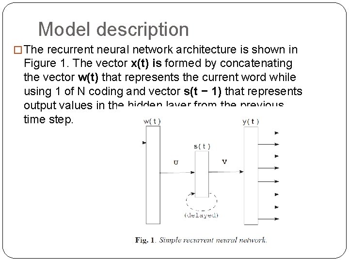
Model description � The recurrent neural network architecture is shown in Figure 1. The vector x(t) is formed by concatenating the vector w(t) that represents the current word while using 1 of N coding and vector s(t − 1) that represents output values in the hidden layer from the previous time step.

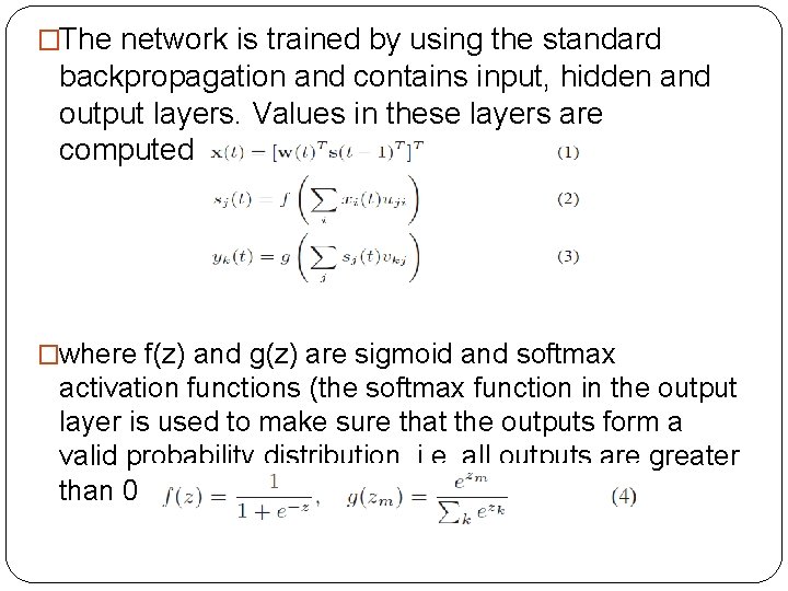
�The network is trained by using the standard backpropagation and contains input, hidden and output layers. Values in these layers are computed as follows: �where f(z) and g(z) are sigmoid and softmax activation functions (the softmax function in the output layer is used to make sure that the outputs form a valid probability distribution, i. e. all outputs are greater than 0 and their sum is 1):

Backpropagation through time �Backpropagation through time (BPTT) can be seen as an extension of the backpropagation algorithm for recurrent networks. �With truncated BPTT, the error is propagated through recurrent connections back in time for a specific number of time steps. �Thus, the network learns to remember information for several time steps in the hidden layer when it is learned by the BPTT.

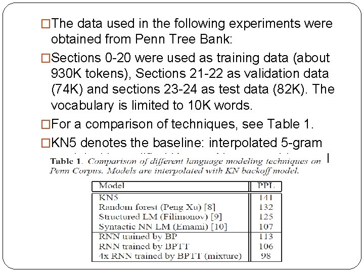
�The data used in the following experiments were obtained from Penn Tree Bank: �Sections 0 -20 were used as training data (about 930 K tokens), Sections 21 -22 as validation data (74 K) and sections 23 -24 as test data (82 K). The vocabulary is limited to 10 K words. �For a comparison of techniques, see Table 1. �KN 5 denotes the baseline: interpolated 5 -gram model with modified Kneser Ney smoothing and no count cutoffs.

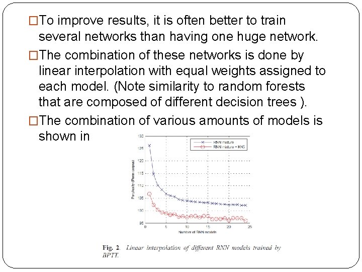
�To improve results, it is often better to train several networks than having one huge network. �The combination of these networks is done by linear interpolation with equal weights assigned to each model. (Note similarity to random forests that are composed of different decision trees ). �The combination of various amounts of models is shown in Figure 2.

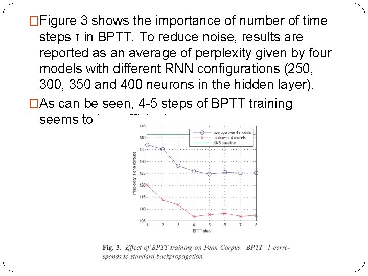
�Figure 3 shows the importance of number of time steps τ in BPTT. To reduce noise, results are reported as an average of perplexity given by four models with different RNN configurations (250, 300, 350 and 400 neurons in the hidden layer). �As can be seen, 4 -5 steps of BPTT training seems to be sufficient.

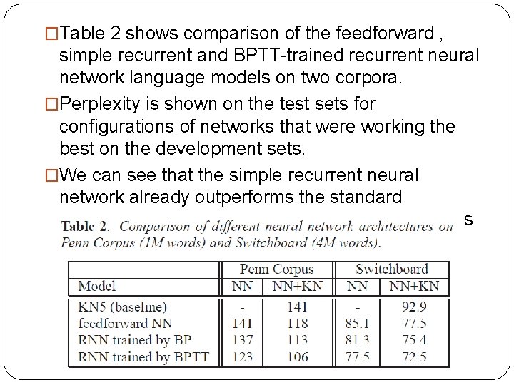
�Table 2 shows comparison of the feedforward , simple recurrent and BPTT-trained recurrent neural network language models on two corpora. �Perplexity is shown on the test sets for configurations of networks that were working the best on the development sets. �We can see that the simple recurrent neural network already outperforms the standard feedforward network, while BPTT training provides another significant improvement.

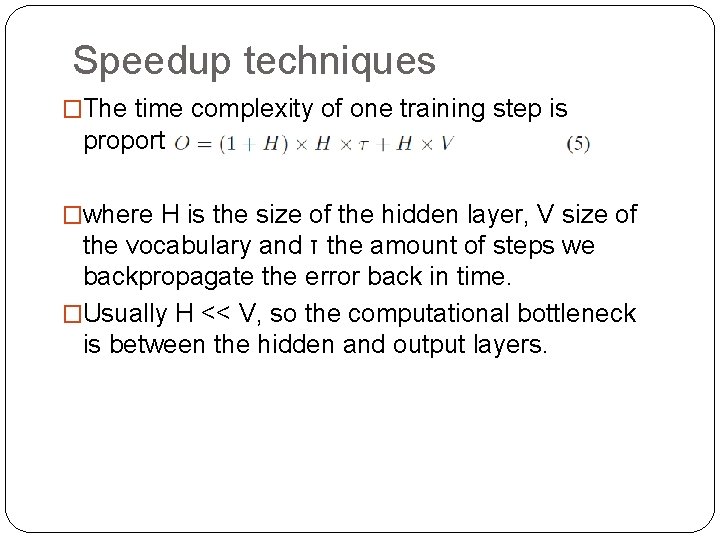
Speedup techniques �The time complexity of one training step is proportional to �where H is the size of the hidden layer, V size of the vocabulary and τ the amount of steps we backpropagate the error back in time. �Usually H << V, so the computational bottleneck is between the hidden and output layers.

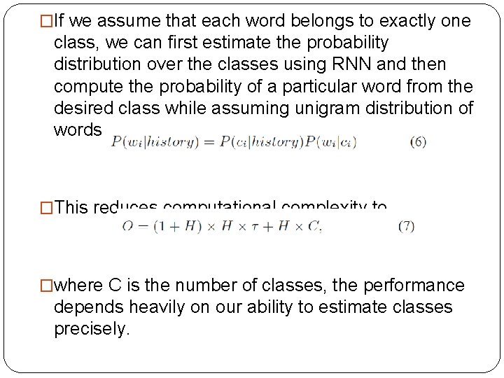
�If we assume that each word belongs to exactly one class, we can first estimate the probability distribution over the classes using RNN and then compute the probability of a particular word from the desired class while assuming unigram distribution of words within the class: �This reduces computational complexity to �where C is the number of classes, the performance depends heavily on our ability to estimate classes precisely.

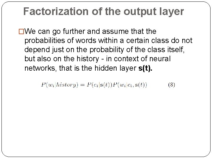
Factorization of the output layer �We can go further and assume that the probabilities of words within a certain class do not depend just on the probability of the class itself, but also on the history - in context of neural networks, that is the hidden layer s(t).

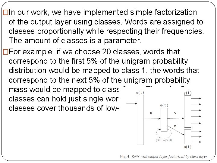
�In our work, we have implemented simple factorization of the output layer using classes. Words are assigned to classes proportionally, while respecting their frequencies. The amount of classes is a parameter. �For example, if we choose 20 classes, words that correspond to the first 5% of the unigram probability distribution would be mapped to class 1, the words that correspond to the next 5% of the unigram probability mass would be mapped to class 2, etc. Thus, the first classes can hold just single words, while the last classes cover thousands of low-frequency words.

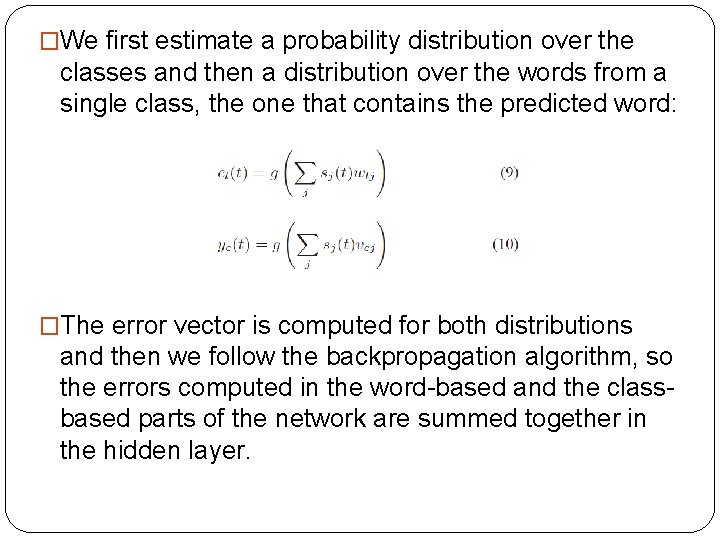
�We first estimate a probability distribution over the classes and then a distribution over the words from a single class, the one that contains the predicted word: �The error vector is computed for both distributions and then we follow the backpropagation algorithm, so the errors computed in the word-based and the classbased parts of the network are summed together in the hidden layer.

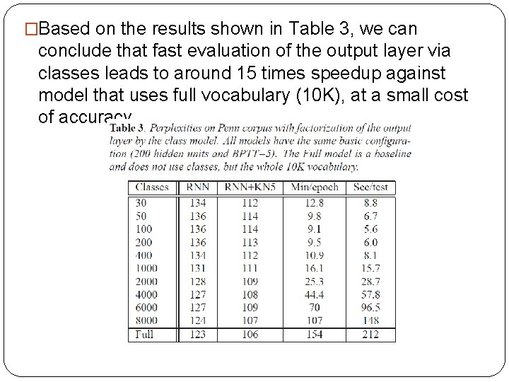
�Based on the results shown in Table 3, we can conclude that fast evaluation of the output layer via classes leads to around 15 times speedup against model that uses full vocabulary (10 K), at a small cost of accuracy.

Conclusion and future work �We presented to our knowledge the first published results when using RNN trained by BPTT in the context of statistical language modeling. �The comparison to standard feedforward neural network based language models, as well as comparison to BP trained RNN models shows clearly the potential of the presented model. �Furthermore, we have shown how to obtain significantly better accuracy of RNN models by combining them linearly. �In the future work, we plan to show to further improve accuracy by combining statically and dynamically evaluated RNN models and by using