ARTIFICIAL NEURAL NETWORKS CSC 576 Data Mining Today

ARTIFICIAL NEURAL NETWORKS CSC 576: Data Mining

Today… Artificial Neural Networks (ANN) Inspiration Perceptron Hidden Nodes Learning

Inspiration Attempts to simulate biological neural systems Animal brains have complex learning systems consisting of closely interconnected sets of neurons

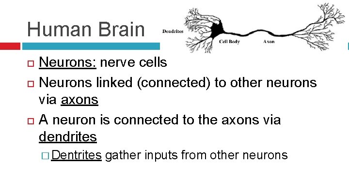
Human Brain Neurons: nerve cells Neurons linked (connected) to other neurons via axons A neuron is connected to the axons via dendrites � Dentrites gather inputs from other neurons

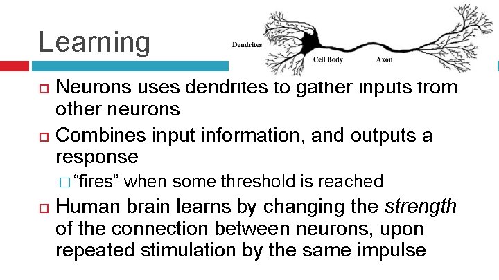
Learning Neurons uses dendrites to gather inputs from other neurons Combines input information, and outputs a response � “fires” when some threshold is reached Human brain learns by changing the strength of the connection between neurons, upon repeated stimulation by the same impulse

Inspiration Human brain contains approximately 1011 neurons Each connected on average to 10, 000 other neurons Total of 1, 000, 000 = 1015 connections

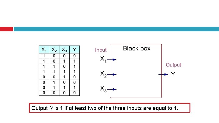
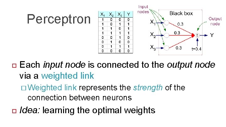
Output Y is 1 if at least two of the three inputs are equal to 1.

Going to begin with simplest model…

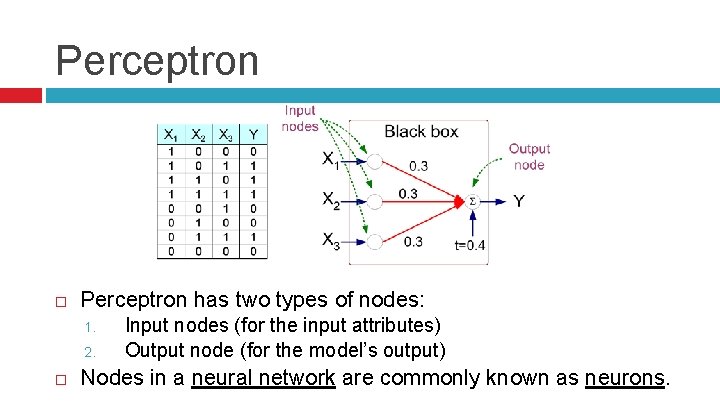
Perceptron has two types of nodes: 1. 2. Input nodes (for the input attributes) Output node (for the model’s output) Nodes in a neural network are commonly known as neurons.

Perceptron Each input node is connected to the output node via a weighted link � Weighted link represents the strength of the connection between neurons Idea: learning the optimal weights

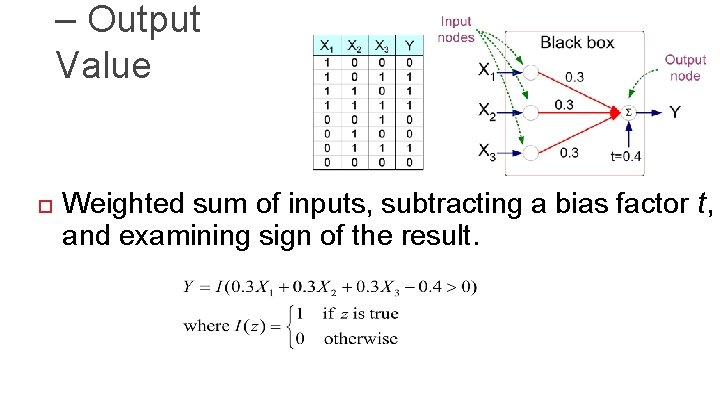
– Output Value Weighted sum of inputs, subtracting a bias factor t, and examining sign of the result.

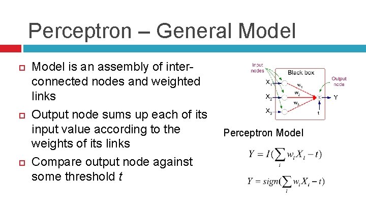
Perceptron – General Model is an assembly of interconnected nodes and weighted links Output node sums up each of its input value according to the weights of its links Compare output node against some threshold t Perceptron Model

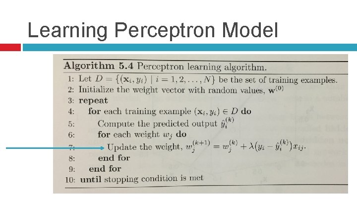
Learning Perceptron Model

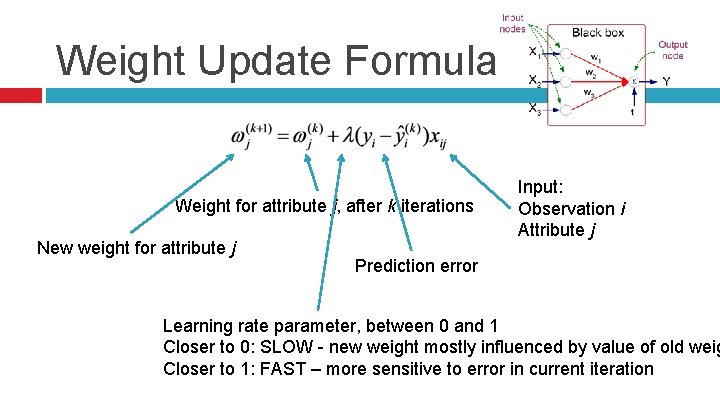
Weight Update Formula Weight for attribute j, after k iterations New weight for attribute j Input: Observation i Attribute j Prediction error Learning rate parameter, between 0 and 1 Closer to 0: SLOW - new weight mostly influenced by value of old weig Closer to 1: FAST – more sensitive to error in current iteration

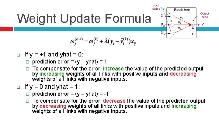
Weight Update Formula If y = +1 and yhat = 0: � � prediction error = (y – yhat) = 1 To compensate for the error: increase the value of the predicted output by increasing weights of all links with positive inputs and decreasing weights of all links with negative inputs. If y = 0 and yhat = 1: � � prediction error = (y – yhat) = -1 To compensate for the error: decrease the value of the predicted output by decreasing weights of all links with positive inputs and increasing weights of all links with negative inputs.

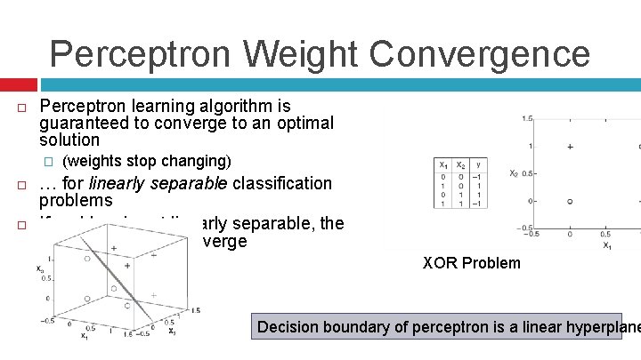
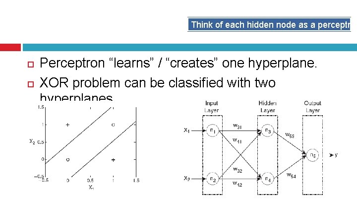
Perceptron Weight Convergence Perceptron learning algorithm is guaranteed to converge to an optimal solution � (weights stop changing) … for linearly separable classification problems If problem is not linearly separable, the algorithm fails to converge XOR Problem Decision boundary of perceptron is a linear hyperplane

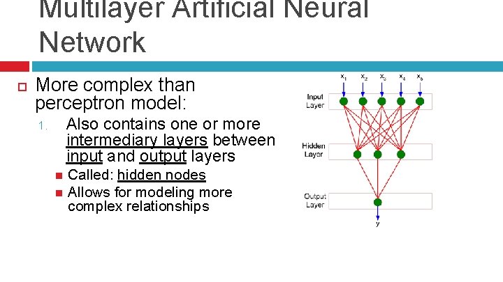
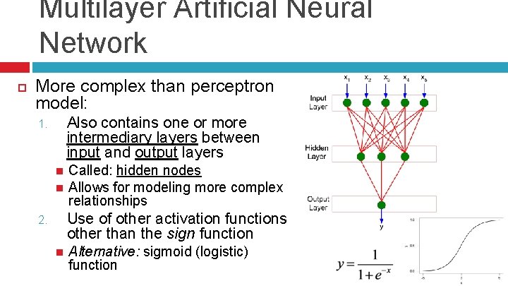
Multilayer Artificial Neural Network More complex than perceptron model: Also contains one or more intermediary layers between input and output layers 1. Called: hidden nodes Allows for modeling more complex relationships

Think of each hidden node as a perceptron Perceptron “learns” / “creates” one hyperplane. XOR problem can be classified with two hyperplanes.

Multilayer Artificial Neural Network More complex than perceptron model: Also contains one or more intermediary layers between input and output layers 1. Called: hidden nodes Allows for modeling more complex relationships Use of other activation functions other than the sign function 2. Alternative: sigmoid (logistic) function

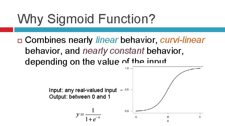
Why Sigmoid Function? Combines nearly linear behavior, curvi-linear behavior, and nearly constant behavior, depending on the value of the input. Input: any real-valued input Output: between 0 and 1

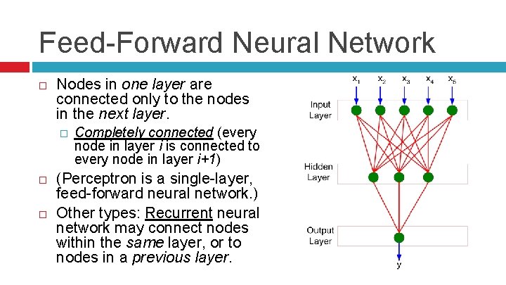
Feed-Forward Neural Network Nodes in one layer are connected only to the nodes in the next layer. � Completely connected (every node in layer i is connected to every node in layer i+1) (Perceptron is a single-layer, feed-forward neural network. ) Other types: Recurrent neural network may connect nodes within the same layer, or to nodes in a previous layer.

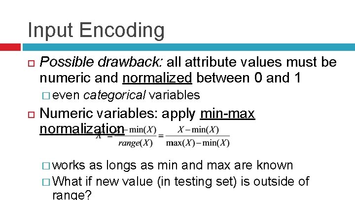
Input Encoding Possible drawback: all attribute values must be numeric and normalized between 0 and 1 � even categorical variables Numeric variables: apply min-max normalization � works as longs as min and max are known � What if new value (in testing set) is outside of range?

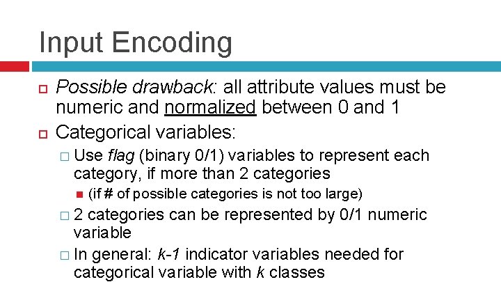
Input Encoding Possible drawback: all attribute values must be numeric and normalized between 0 and 1 Categorical variables: � Use flag (binary 0/1) variables to represent each category, if more than 2 categories � 2 (if # of possible categories is not too large) categories can be represented by 0/1 numeric variable � In general: k-1 indicator variables needed for categorical variable with k classes

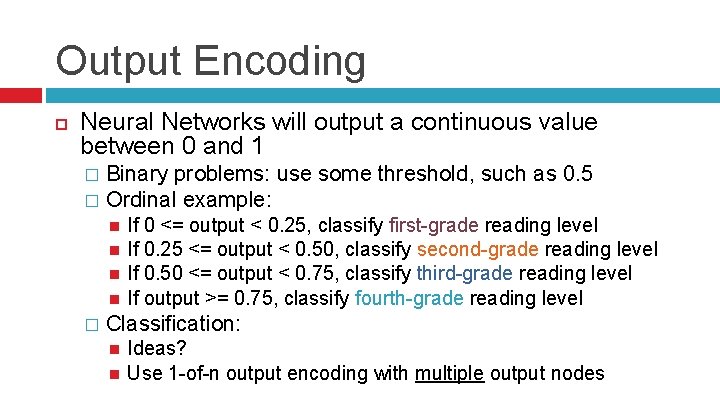
Output Encoding Neural Networks will output a continuous value between 0 and 1 Binary problems: use some threshold, such as 0. 5 � Ordinal example: � � If 0 <= output < 0. 25, classify first-grade reading level If 0. 25 <= output < 0. 50, classify second-grade reading level If 0. 50 <= output < 0. 75, classify third-grade reading level If output >= 0. 75, classify fourth-grade reading level Classification: Ideas? Use 1 -of-n output encoding with multiple output nodes

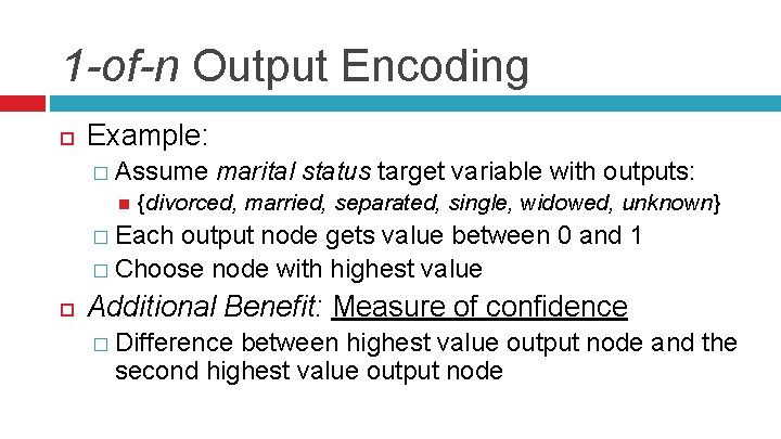
1 -of-n Output Encoding Example: � Assume marital status target variable with outputs: {divorced, married, separated, single, widowed, unknown} � Each output node gets value between 0 and 1 � Choose node with highest value Additional Benefit: Measure of confidence � Difference between highest value output node and the second highest value output node

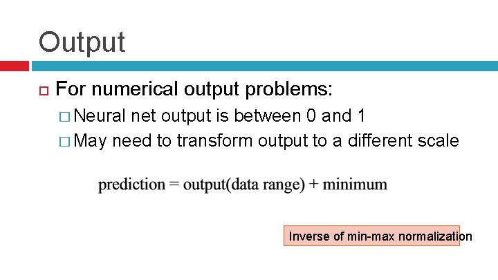
Output For numerical output problems: � Neural net output is between 0 and 1 � May need to transform output to a different scale Inverse of min-max normalization

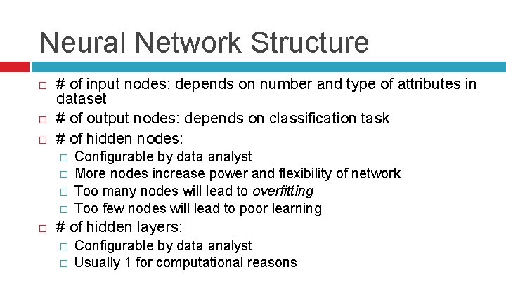
Neural Network Structure # of input nodes: depends on number and type of attributes in dataset # of output nodes: depends on classification task # of hidden nodes: � � Configurable by data analyst More nodes increase power and flexibility of network Too many nodes will lead to overfitting Too few nodes will lead to poor learning # of hidden layers: � � Configurable by data analyst Usually 1 for computational reasons

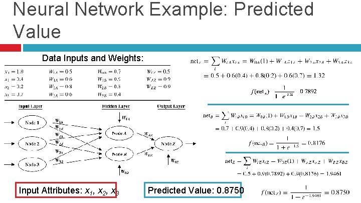
Neural Network Example: Predicted Value Data Inputs and Weights: Input Attributes: x 1, x 2, x 3 Predicted Value: 0. 8750

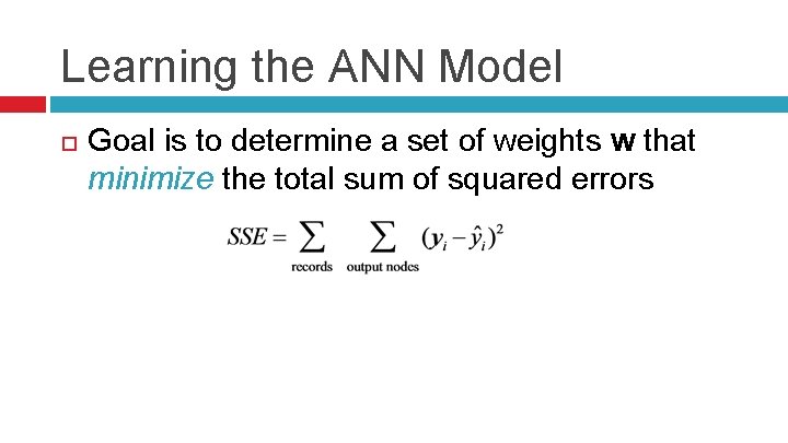
Learning the ANN Model Goal is to determine a set of weights w that minimize the total sum of squared errors

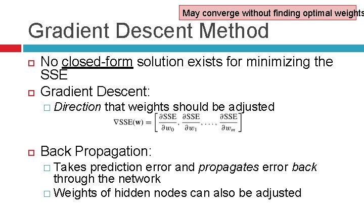
May converge without finding optimal weights Gradient Descent Method No closed-form solution exists for minimizing the SSE Gradient Descent: � Direction that weights should be adjusted Back Propagation: � Takes prediction error and propagates error back through the network � Weights of hidden nodes can also be adjusted

Learning the ANN Model Keep adjusting weights until some stopping criterion is met: 1. 2. 3. 4. SSE reduced below some threshold Weights are not changing anymore Elapsed training time exceeds limit Number of iterations exceeds limits

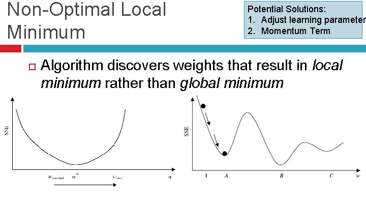
Non-Optimal Local Minimum Potential Solutions: 1. Adjust learning parameter 2. Momentum Term Algorithm discovers weights that result in local minimum rather than global minimum

Characteristics of Artificial Neural Networks Important to choose appropriate network topology Very expensive hypothesis space � Fast classification time Can handle redundant features � Weights for redundant features tend to be very small Gradient descent for learning weights may converge to local minimum � � Relatively lengthy training time Use momentum term Learn multiple models (remember initial weights are random) Interpretability: what do weights of hidden nodes mean?

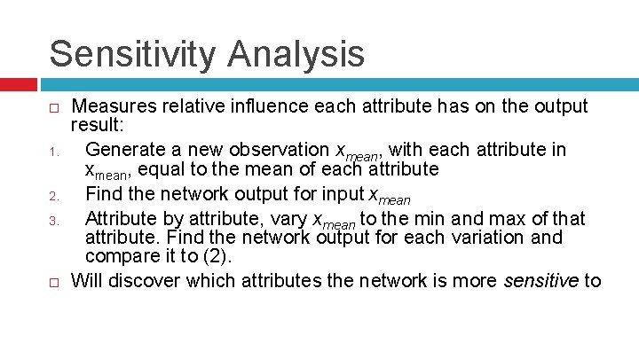
Sensitivity Analysis 1. 2. 3. Measures relative influence each attribute has on the output result: Generate a new observation xmean, with each attribute in xmean, equal to the mean of each attribute Find the network output for input xmean Attribute by attribute, vary xmean to the min and max of that attribute. Find the network output for each variation and compare it to (2). Will discover which attributes the network is more sensitive to

References Data Science from Scratch, 1 st Edition, Grus Introduction to Data Mining, 1 st edition, Tan et al. Discovering Knowledge in Data, 2 nd edition, Larose et al.