Artificial Neural Networks Artificial neural networks ANNs provide

![Perceptron Learning Rule t=-1 t=1 o=1 w=[0. 25, – 0. 1, 0. 5] x Perceptron Learning Rule t=-1 t=1 o=1 w=[0. 25, – 0. 1, 0. 5] x](https://slidetodoc.com/presentation_image_h/23f81a9a2be5b4e14898aed3c9584ea1/image-13.jpg)
![Incremental (Stochastic) Gradient Descent • Batch mode : gradient descent w=w - ED[w] over Incremental (Stochastic) Gradient Descent • Batch mode : gradient descent w=w - ED[w] over](https://slidetodoc.com/presentation_image_h/23f81a9a2be5b4e14898aed3c9584ea1/image-23.jpg)

- Slides: 39

Artificial Neural Networks • Artificial neural networks (ANNs) provide a general, practical method for learning real-valued, discrete-valued, and vector-valued functions from examples. • Algorithms such as BACKPROPAGATION gradient descent to tune network parameters to best fit a training set of input-output pairs. • ANN learning is robust to errors in the training data and has been successfully applied to problems such as interpreting visual scenes, speech recognition, and learning robot control strategies. CS 464 Introduction to Machine Learning 1

Biological Motivation • The study of artificial neural networks (ANNs) has been inspired in part by the observation that biological learning systems are built of very complex webs of interconnected neurons. • Artificial neural networks are built out of a densely interconnected set of simple units, where each unit takes a number of real-valued inputs (possibly the outputs of other units) and produces a single real-valued output (which may become the input to many other units). • The human brain is estimated to contain a densely interconnected network of approximately 1011 neurons, each connected, on average, to 104 others. – Neuron activity is typically inhibited through connections to other neurons. CS 464 Introduction to Machine Learning 2

ALVINN – Neural Network Learning To Steer An Autonomous Vehicle CS 464 Introduction to Machine Learning 3

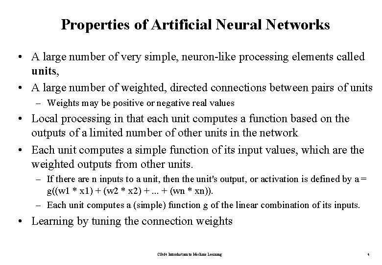
Properties of Artificial Neural Networks • A large number of very simple, neuron-like processing elements called units, • A large number of weighted, directed connections between pairs of units – Weights may be positive or negative real values • Local processing in that each unit computes a function based on the outputs of a limited number of other units in the network • Each unit computes a simple function of its input values, which are the weighted outputs from other units. – If there are n inputs to a unit, then the unit's output, or activation is defined by a = g((w 1 * x 1) + (w 2 * x 2) +. . . + (wn * xn)). – Each unit computes a (simple) function g of the linear combination of its inputs. • Learning by tuning the connection weights CS 464 Introduction to Machine Learning 4

Appropriate Problems for NN Learning • Instances are represented by many attribute-value pairs. • The target function output may be discrete-valued, real-valued, or a vector of several real-valued or discrete-valued attributes. • The training examples may contain errors. • Long training times are acceptable. • Fast evaluation of the learned target function may be required. • The ability of humans to understand the learned target function is not important. CS 464 Introduction to Machine Learning 5

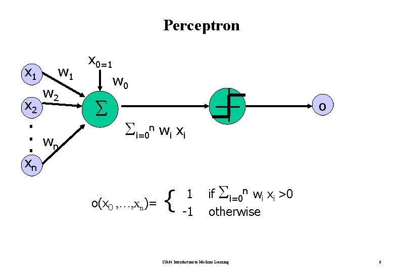
Perceptron x 1 x 2 . . . w 1 w 2 wn x 0=1 w 0 o i=0 n wi xi xn o(x 0 , …, xn)= { 1 -1 if i=0 n wi xi >0 otherwise CS 464 Introduction to Machine Learning 6

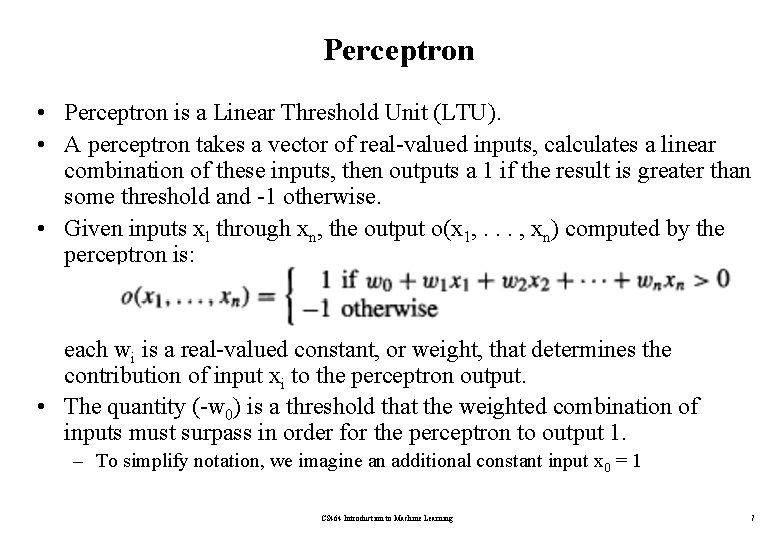
Perceptron • Perceptron is a Linear Threshold Unit (LTU). • A perceptron takes a vector of real-valued inputs, calculates a linear combination of these inputs, then outputs a 1 if the result is greater than some threshold and -1 otherwise. • Given inputs xl through xn, the output o(x 1, . . . , xn) computed by the perceptron is: each wi is a real-valued constant, or weight, that determines the contribution of input xi to the perceptron output. • The quantity (-w 0) is a threshold that the weighted combination of inputs must surpass in order for the perceptron to output 1. – To simplify notation, we imagine an additional constant input x 0 = 1 CS 464 Introduction to Machine Learning 7

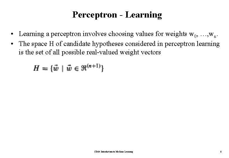
Perceptron - Learning • Learning a perceptron involves choosing values for weights w 0, …, wn. • The space H of candidate hypotheses considered in perceptron learning is the set of all possible real-valued weight vectors CS 464 Introduction to Machine Learning 8

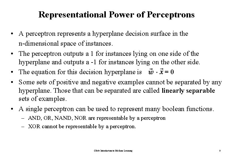
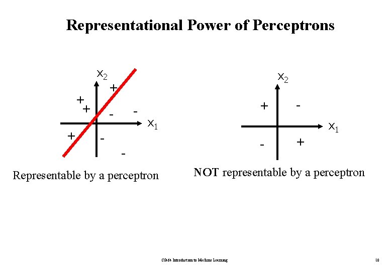
Representational Power of Perceptrons • A perceptron represents a hyperplane decision surface in the n-dimensional space of instances. • The perceptron outputs a 1 for instances lying on one side of the hyperplane and outputs a -1 for instances lying on the other side. • The equation for this decision hyperplane is =0 • Some sets of positive and negative examples cannot be separated by any hyperplane. Those that can be separated are called linearly separable sets of examples. • A single perceptron can be used to represent many boolean functions. – AND, OR, NAND, NOR are representable by a perceptron – XOR cannot be representable by a perceptron. CS 464 Introduction to Machine Learning 9

Representational Power of Perceptrons x 2 + + + x 2 + - - + - x 1 - - Representable by a perceptron + NOT representable by a perceptron CS 464 Introduction to Machine Learning 10

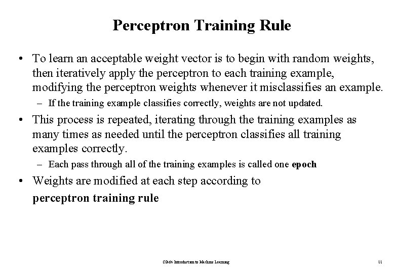
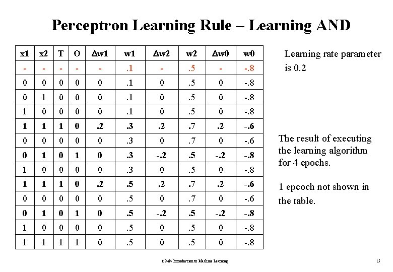
Perceptron Training Rule • To learn an acceptable weight vector is to begin with random weights, then iteratively apply the perceptron to each training example, modifying the perceptron weights whenever it misclassifies an example. – If the training example classifies correctly, weights are not updated. • This process is repeated, iterating through the training examples as many times as needed until the perceptron classifies all training examples correctly. – Each pass through all of the training examples is called one epoch • Weights are modified at each step according to perceptron training rule CS 464 Introduction to Machine Learning 11

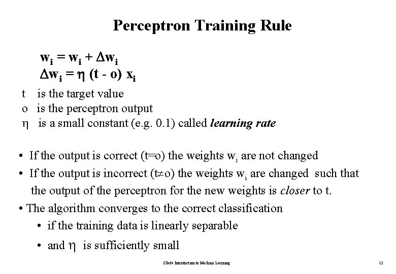
Perceptron Training Rule wi = wi + wi wi = (t - o) xi t is the target value o is the perceptron output is a small constant (e. g. 0. 1) called learning rate • If the output is correct (t=o) the weights wi are not changed • If the output is incorrect (t o) the weights wi are changed such that the output of the perceptron for the new weights is closer to t. • The algorithm converges to the correct classification • if the training data is linearly separable • and is sufficiently small CS 464 Introduction to Machine Learning 12
![Perceptron Learning Rule t1 t1 o1 w0 25 0 1 0 5 x Perceptron Learning Rule t=-1 t=1 o=1 w=[0. 25, – 0. 1, 0. 5] x](https://slidetodoc.com/presentation_image_h/23f81a9a2be5b4e14898aed3c9584ea1/image-13.jpg)
Perceptron Learning Rule t=-1 t=1 o=1 w=[0. 25, – 0. 1, 0. 5] x 2 = 0. 2 x 1 – 0. 5 o=-1 (x, t)=([2, 1], -1) (x, t)=([-1, -1], 1) (x, t)=([1, 1], 1) o=sgn(0. 45 -0. 6+0. 3)=1 o=sgn(0. 25+0. 1 -0. 5) o=sgn(0. 25 -0. 7+0. 1)=-1 w=[0. 2 – 0. 2] w=[-0. 2, – 0. 4, – 0. 2] w=[0. 2, 0. 2] CS 464 Introduction to Machine Learning 13

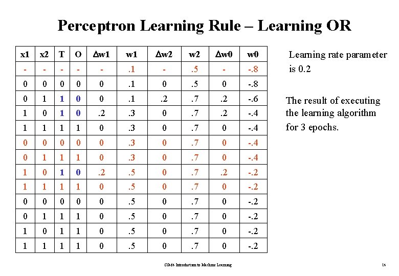
Perceptron Learning Rule – Learning OR x 1 x 2 T O w 1 w 2 w 0 - - - . 1 - . 5 - -. 8 0 0 0 . 1 0 . 5 0 -. 8 0 1 1 0 0 . 1 . 2 . 7 . 2 -. 6 1 0 . 2 . 3 0 . 7 . 2 -. 4 1 1 0 . 3 0 . 7 0 -. 4 0 0 0 . 3 0 . 7 0 -. 4 0 1 1 1 0 . 3 0 . 7 0 -. 4 1 0 . 2 . 5 0 . 7 . 2 -. 2 1 1 0 . 5 0 . 7 0 -. 2 0 0 0 . 5 0 . 7 0 -. 2 0 1 1 1 0 . 5 0 . 7 0 -. 2 1 0 1 1 0 . 5 0 . 7 0 -. 2 CS 464 Introduction to Machine Learning rate parameter is 0. 2 The result of executing the learning algorithm for 3 epochs. 14

Perceptron Learning Rule – Learning AND x 1 x 2 T O w 1 w 2 w 0 - - - . 1 - . 5 - -. 8 0 0 0 . 1 0 . 5 0 -. 8 0 1 0 0 0 . 1 0 . 5 0 -. 8 1 1 1 0 . 2 . 3 . 2 . 7 . 2 -. 6 0 0 0 . 3 0 . 7 0 -. 6 0 1 0 . 3 -. 2 . 5 -. 2 -. 8 1 0 0 . 3 0 . 5 0 -. 8 1 1 1 0 . 2 . 5 . 2 . 7 . 2 -. 6 0 0 0 . 5 0 . 7 0 -. 6 0 1 0 . 5 -. 2 -. 8 1 0 0 . 5 0 -. 8 1 1 0 . 5 0 -. 8 CS 464 Introduction to Machine Learning rate parameter is 0. 2 The result of executing the learning algorithm for 4 epochs. 1 epcoch not shown in the table. 15

Gradient Descent and the Delta Rule • The perceptron rule finds a successful weight vector when the training examples are linearly separable, it can fail to converge if the examples are not linearly separable. • The delta rule overcomes this difficulty. • If the training examples are not linearly separable, the delta rule converges toward a best-fit approximation to the target concept. • The key idea behind the delta rule is to use gradient descent to search the hypothesis space of possible weight vectors to find the weights that best fit the training examples. • The delta rule is important because gradient descent provides the basis for the BACKPROPAGATION Algorithm, which can learn networks with many interconnected units. – The gradient descent can serve as the basis for learning algorithms that must search through hypothesis spaces containing many different types of continuously parameterized hypotheses CS 464 Introduction to Machine Learning 16

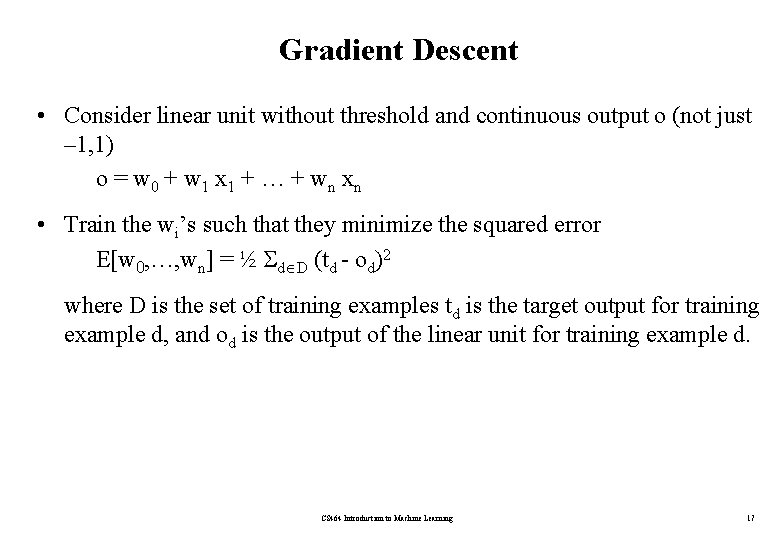
Gradient Descent • Consider linear unit without threshold and continuous output o (not just – 1, 1) o = w 0 + w 1 x 1 + … + wn xn • Train the wi’s such that they minimize the squared error E[w 0, …, wn] = ½ d D (td - od)2 where D is the set of training examples td is the target output for training example d, and od is the output of the linear unit for training example d. CS 464 Introduction to Machine Learning 17

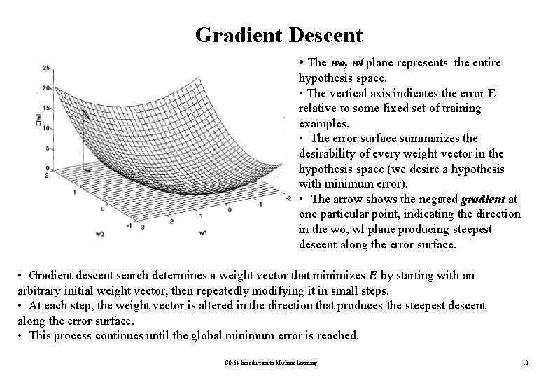
Gradient Descent • The wo, wl plane represents the entire hypothesis space. • The vertical axis indicates the error E relative to some fixed set of training examples. • The error surface summarizes the desirability of every weight vector in the hypothesis space (we desire a hypothesis with minimum error). • The arrow shows the negated gradient at one particular point, indicating the direction in the wo, wl plane producing steepest descent along the error surface. • Gradient descent search determines a weight vector that minimizes E by starting with an arbitrary initial weight vector, then repeatedly modifying it in small steps. • At each step, the weight vector is altered in the direction that produces the steepest descent along the error surface. • This process continues until the global minimum error is reached. CS 464 Introduction to Machine Learning 18

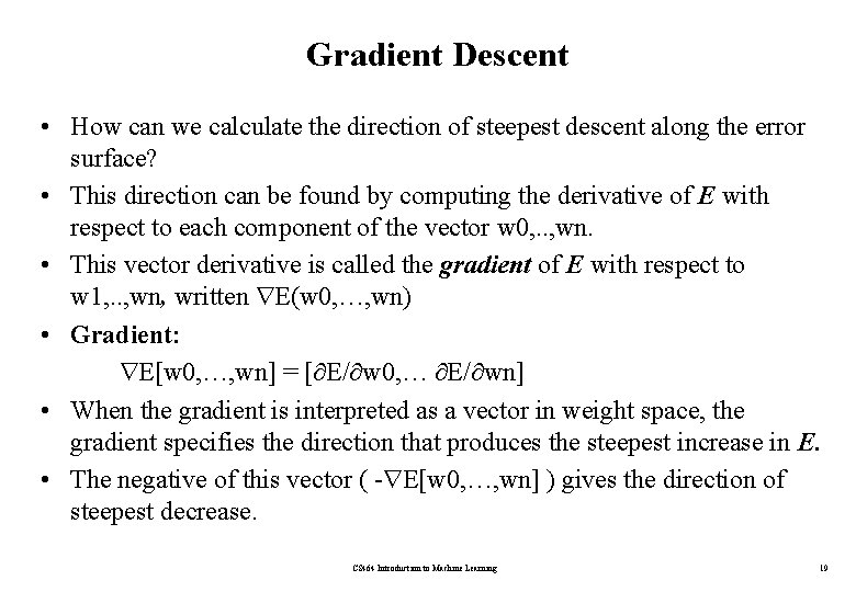
Gradient Descent • How can we calculate the direction of steepest descent along the error surface? • This direction can be found by computing the derivative of E with respect to each component of the vector w 0, . . , wn. • This vector derivative is called the gradient of E with respect to w 1, . . , wn, written E(w 0, …, wn) • Gradient: E[w 0, …, wn] = [ E/ w 0, … E/ wn] • When the gradient is interpreted as a vector in weight space, the gradient specifies the direction that produces the steepest increase in E. • The negative of this vector ( - E[w 0, …, wn] ) gives the direction of steepest decrease. CS 464 Introduction to Machine Learning 19

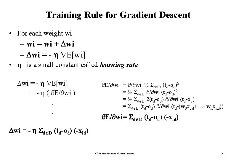
Training Rule for Gradient Descent • For each weight wi – wi = wi + wi – wi = - E[wi] • is a small constant called learning rate wi = - E[wi] = - ( E/ wi ). . E/ wi = / wi ½ d D (td-od)2 = ½ d D / wi (td-od)2 = ½ d D 2(td-od) / wi (td-od) = d D (td-od) / wi (td-(w 0 x 0 d+…+wnxnd)) E/ wi= d D (td-od) (-xid) wi = - d D (td-od) (-xid) CS 464 Introduction to Machine Learning 20

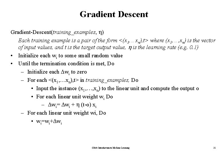
Gradient Descent Gradient-Descent(training_examples, ) Each training example is a pair of the form <(x 1, …xn), t> where (x 1, …, xn) is the vector of input values, and t is the target output value, is the learning rate (e. g. 0. 1) • Initialize each wi to some small random value • Until the termination condition is met, Do – Initialize each wi to zero – For each <(x 1, …xn), t> in training_examples, Do • Input the instance (x 1, …, xn) to the linear unit and compute the output o • For each linear unit weight wi Do – wi= wi + (t-o) xi – For each linear unit weight wi, Do • wi=wi+ wi CS 464 Introduction to Machine Learning 21

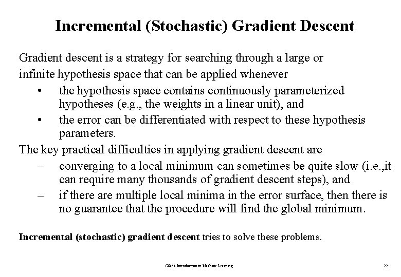
Incremental (Stochastic) Gradient Descent Gradient descent is a strategy for searching through a large or infinite hypothesis space that can be applied whenever • the hypothesis space contains continuously parameterized hypotheses (e. g. , the weights in a linear unit), and • the error can be differentiated with respect to these hypothesis parameters. The key practical difficulties in applying gradient descent are – converging to a local minimum can sometimes be quite slow (i. e. , it can require many thousands of gradient descent steps), and – if there are multiple local minima in the error surface, then there is no guarantee that the procedure will find the global minimum. Incremental (stochastic) gradient descent tries to solve these problems. CS 464 Introduction to Machine Learning 22
![Incremental Stochastic Gradient Descent Batch mode gradient descent ww EDw over Incremental (Stochastic) Gradient Descent • Batch mode : gradient descent w=w - ED[w] over](https://slidetodoc.com/presentation_image_h/23f81a9a2be5b4e14898aed3c9584ea1/image-23.jpg)
Incremental (Stochastic) Gradient Descent • Batch mode : gradient descent w=w - ED[w] over the entire data D ED[w]=1/2 d(td-od)2 • Incremental mode: gradient descent w=w - Ed[w] over individual training examples d Ed[w]=1/2 (td-od)2 Incremental Gradient Descent can approximate Batch Gradient Descent arbitrarily closely if is small enough CS 464 Introduction to Machine Learning 23

Incremental (Stochastic) Gradient Descent Incremental (Stochastic) Gradient-Descent(training_examples, ) Each training example is a pair of the form <(x 1, …xn), t> where (x 1, …, xn) is the vector of input values, and t is the target output value, is the learning rate (e. g. 0. 1) • Initialize each wi to some small random value • Until the termination condition is met, Do – Initialize / / / each / / w / /i to / / zero ///// – For each <(x 1, …xn), t> in training_examples, Do • Input the instance (x 1, …, xn) to the linear unit and compute the output o • For each linear unit weight wi Do / /–/ / w / /i=/ w / / /i +/ / /(t-o) / / /x/i / / wi= wi + (t-o) xi – For / / /each / / / linear / / unit / / / weight / / /wi, / / Do /// / • / /w/i=w / / i/+ w / / /i / / / / / CS 464 Introduction to Machine Learning 24

Incremental (Stochastic) Gradient Descent • In standard gradient descent, the error is summed over all examples before updating weights, whereas in stochastic gradient descent weights are updated upon examining each training example. • Summing over multiple examples in standard gradient descent requires more computation per weight update step. On the other hand, because it uses the true gradient, standard gradient descent is often used with a larger step size per weight update than stochastic gradient descent. • In cases where there are multiple local minima with respect to E(w 0, …, wn), stochastic gradient descent can sometimes avoid falling into these local minima because it uses the various Ed(w 0, …, wn) rather than E (w 0, …, wn) to guide its search. CS 464 Introduction to Machine Learning 25

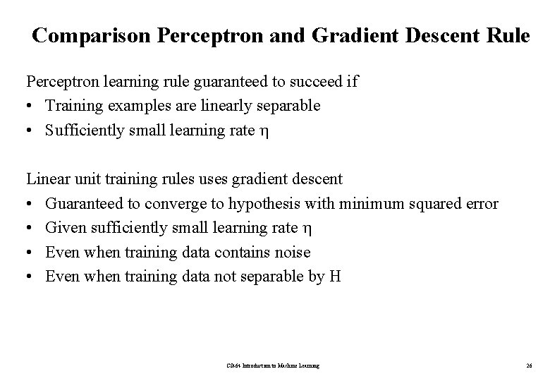
Comparison Perceptron and Gradient Descent Rule Perceptron learning rule guaranteed to succeed if • Training examples are linearly separable • Sufficiently small learning rate Linear unit training rules uses gradient descent • Guaranteed to converge to hypothesis with minimum squared error • Given sufficiently small learning rate • Even when training data contains noise • Even when training data not separable by H CS 464 Introduction to Machine Learning 26

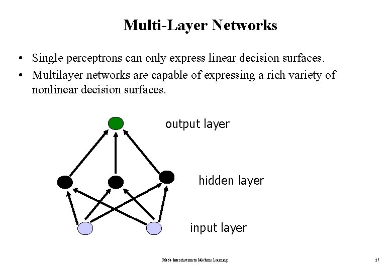
Multi-Layer Networks • Single perceptrons can only express linear decision surfaces. • Multilayer networks are capable of expressing a rich variety of nonlinear decision surfaces. output layer hidden layer input layer CS 464 Introduction to Machine Learning 27

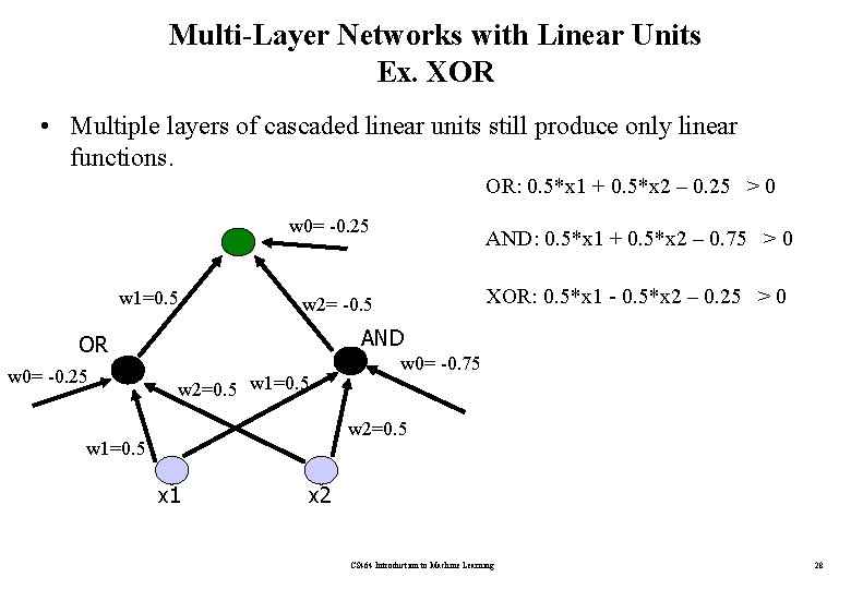
Multi-Layer Networks with Linear Units Ex. XOR • Multiple layers of cascaded linear units still produce only linear functions. OR: 0. 5*x 1 + 0. 5*x 2 – 0. 25 > 0 w 0= -0. 25 w 1=0. 5 XOR: 0. 5*x 1 - 0. 5*x 2 – 0. 25 > 0 w 2= -0. 5 AND OR w 0= -0. 25 AND: 0. 5*x 1 + 0. 5*x 2 – 0. 75 > 0 w 2=0. 5 w 1=0. 5 w 0= -0. 75 w 2=0. 5 w 1=0. 5 x 1 x 2 CS 464 Introduction to Machine Learning 28

Multi-Layer Networks with Non-Linear Units • Multiple layers of cascaded linear units still produce only linear functions. • We prefer networks capable of representing highly nonlinear functions. • What we need is a unit whose output is a nonlinear function of its inputs, but whose output is also a differentiable function of its inputs. • One solution is the sigmoid unit, a unit very much like a perceptron, but based on a smoothed, differentiable threshold function. CS 464 Introduction to Machine Learning 29

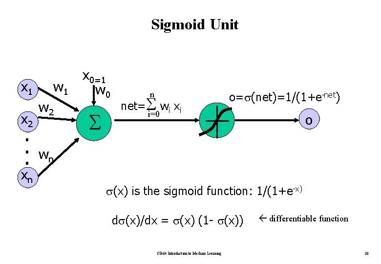
Sigmoid Unit x 1 x 2 . . . xn w 1 w 2 x 0=1 w 0 n net= wi xi o= (net)=1/(1+e-net) i=0 o wn (x) is the sigmoid function: 1/(1+e-x) d (x)/dx = (x) (1 - (x)) CS 464 Introduction to Machine Learning differentiable function 30

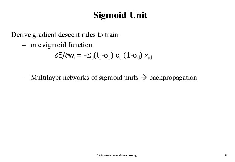
Sigmoid Unit Derive gradient descent rules to train: – one sigmoid function E/ wi = - d(td-od) od (1 -od) xid – Multilayer networks of sigmoid units backpropagation CS 464 Introduction to Machine Learning 31

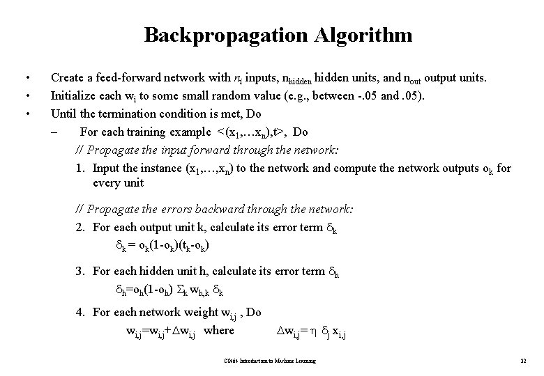
Backpropagation Algorithm • • • Create a feed-forward network with ni inputs, nhidden units, and nout output units. Initialize each wi to some small random value (e. g. , between -. 05 and. 05). Until the termination condition is met, Do – For each training example <(x 1, …xn), t>, Do // Propagate the input forward through the network: 1. Input the instance (x 1, …, xn) to the network and compute the network outputs ok for every unit // Propagate the errors backward through the network: 2. For each output unit k, calculate its error term k k = ok(1 -ok)(tk-ok) 3. For each hidden unit h, calculate its error term h h=oh(1 -oh) k wh, k k 4. For each network weight wi, j , Do wi, j=wi, j+ wi, j where wi, j= j xi, j CS 464 Introduction to Machine Learning 32

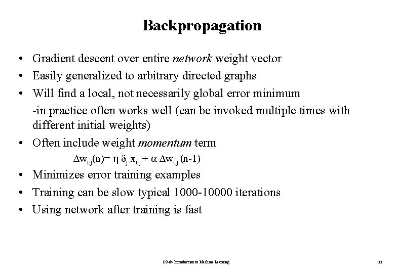
Backpropagation • Gradient descent over entire network weight vector • Easily generalized to arbitrary directed graphs • Will find a local, not necessarily global error minimum -in practice often works well (can be invoked multiple times with different initial weights) • Often include weight momentum term wi, j(n)= j xi, j + wi, j (n-1) • Minimizes error training examples • Training can be slow typical 1000 -10000 iterations • Using network after training is fast CS 464 Introduction to Machine Learning 33

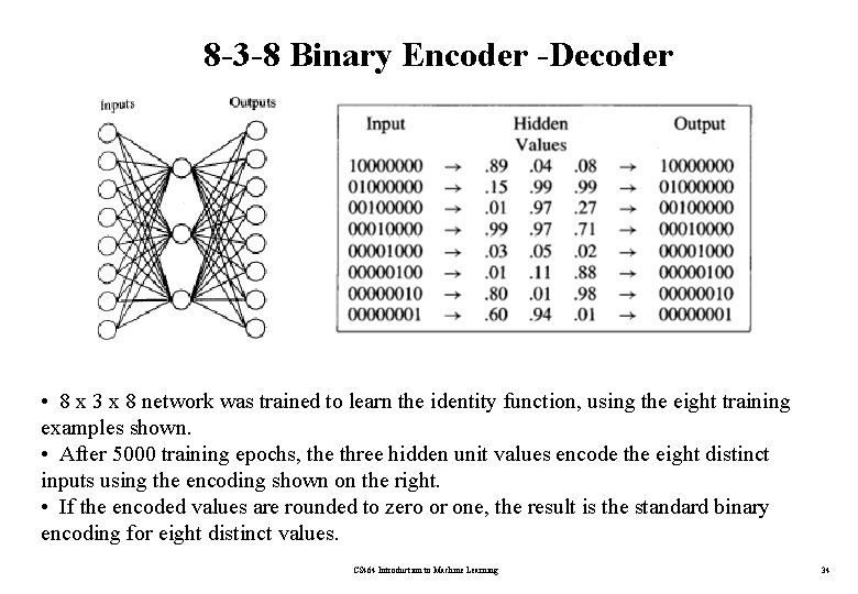
8 -3 -8 Binary Encoder -Decoder • 8 x 3 x 8 network was trained to learn the identity function, using the eight training examples shown. • After 5000 training epochs, the three hidden unit values encode the eight distinct inputs using the encoding shown on the right. • If the encoded values are rounded to zero or one, the result is the standard binary encoding for eight distinct values. CS 464 Introduction to Machine Learning 34

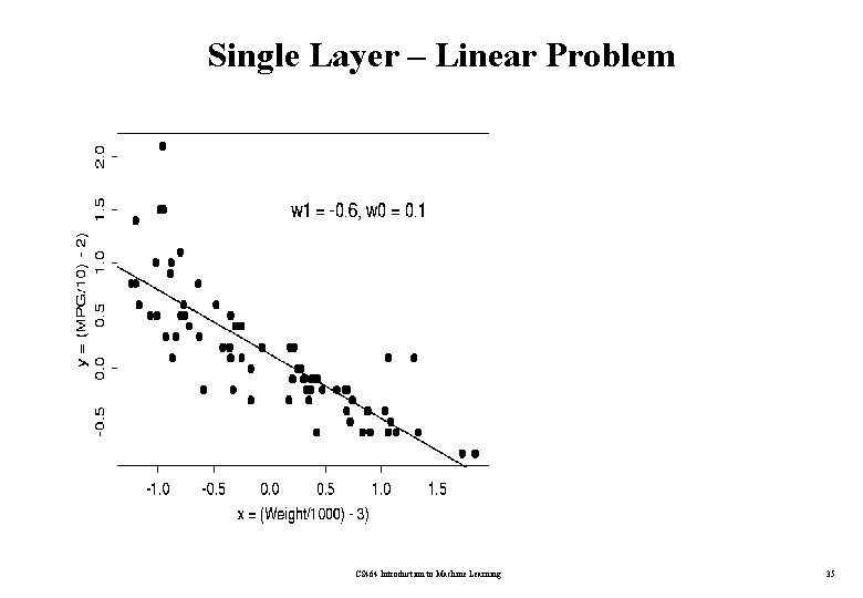
Single Layer – Linear Problem CS 464 Introduction to Machine Learning 35

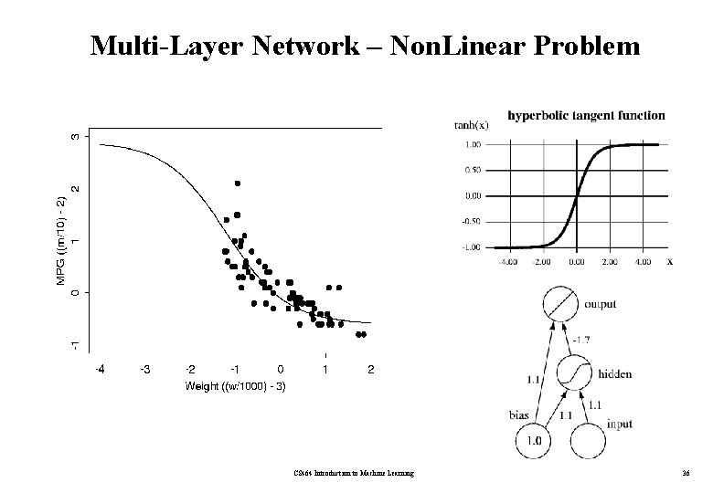
Multi-Layer Network – Non. Linear Problem CS 464 Introduction to Machine Learning 36

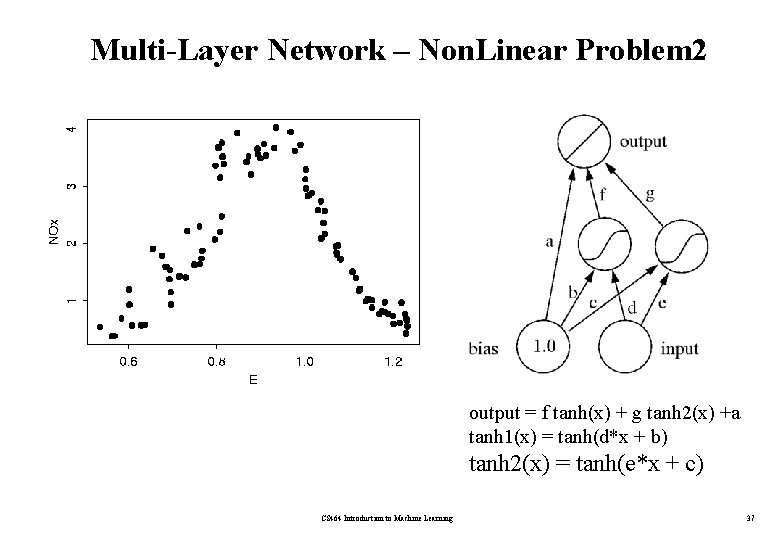
Multi-Layer Network – Non. Linear Problem 2 output = f tanh(x) + g tanh 2(x) +a tanh 1(x) = tanh(d*x + b) tanh 2(x) = tanh(e*x + c) CS 464 Introduction to Machine Learning 37

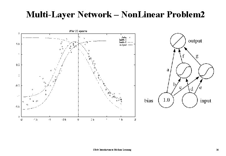
Multi-Layer Network – Non. Linear Problem 2 CS 464 Introduction to Machine Learning 38

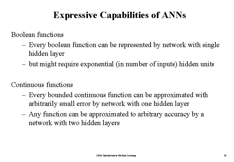
Expressive Capabilities of ANNs Boolean functions – Every boolean function can be represented by network with single hidden layer – but might require exponential (in number of inputs) hidden units Continuous functions – Every bounded continuous function can be approximated with arbitrarily small error by network with one hidden layer – Any function can be approximated to arbitrary accuracy by a network with two hidden layers CS 464 Introduction to Machine Learning 39