Supervised Learning Artificial Neural Networks Artificial Neural Networks

Supervised Learning Artificial Neural Networks

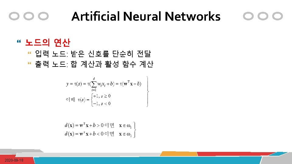
Artificial Neural Networks 인간의 뇌 신경망을 모방 입력 출력

Artificial Neural Networks 구성 요소 Activation function Network topology (or architecture) Neuron 수, Layer 수 Training algorithm Neuron 간 weight를 설정하는 알고리즘

Artificial Neural Networks Activation functions Unit step function Sigmoid function Commonly used Differentiable (미분가능): Weight 최적화를 위 해 중요한 성질

Artificial Neural Networks Network topology Layer의 수 Network 정보의 backward flow 여부 각 layer의 노드 수

Artificial Neural Networks Network topology Single-layer network 기초적인 패턴 classification에 활용 특히, linearly separable patterns Multi-layer network Hidden layer 포함

Artificial Neural Networks Network topology Deep Neural Network: 다수의 hidden layer를 가짐 => Deep Learning

Artificial Neural Networks Network topology Feed-forward network multilayer feedforward network (or Multilayer Perceptron, MLP): ANN의 표준 Feedback (or recurrent) network allows extremely complex patterns to be learned used for stock market prediction, speech comprehension, or weather forecasting Short-term memory

Artificial Neural Networks Network topology Input layer의 노드 수: 입력데이터의 feature 수를 가지고 결정 Output layer의 노드 수: class 컬럼의 level 수를 가지고 결정 Hidden layer의 노드 수: 마땅한 결정 인자가 없음

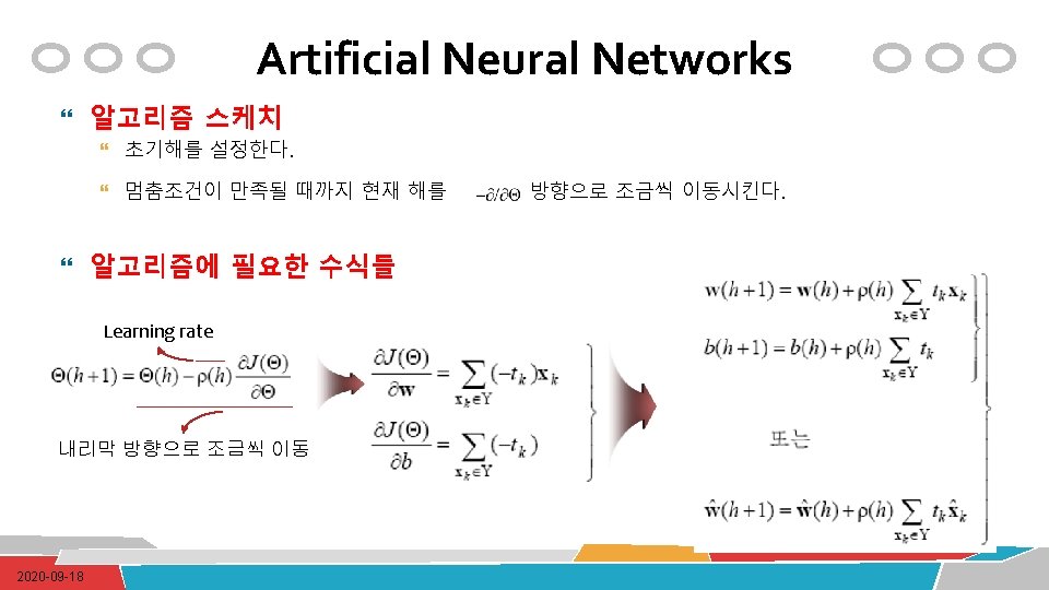
Artificial Neural Networks Training algorithm Backpropagation 기법

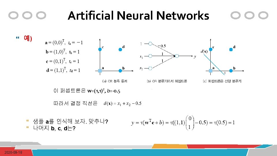
Artificial Neural Networks 퍼셉트론 학습 a=(0, 0)T b=(1, 0)T c=(0, 1)T d=(1, 1)T ta= -1 tb= -1 tc= -1 td=1 예) AND 분류 문제 c d 1 x 1 a 2020 -09 -18 b x 2 ? ? ? y

Artificial Neural Networks 예) OR 분류 문제 w(0)=(-0. 5, 0. 75)T, b(0)=0. 375 ① d(x)= -0. 5 x 1+0. 75 x 2+0. 375 Y={a, b} ② d(x)= -0. 1 x 1+0. 75 x 2+0. 375 Y={a} 2020 -09 -18

Artificial Neural Networks A dataset Fields 1. 4 2. 7 1. 9 3. 8 3. 4 3. 2 6. 4 2. 8 1. 7 4. 1 0. 2 etc … class 0 0 1 0

Artificial Neural Networks Training the neural network Fields class 1. 4 2. 7 1. 9 0 3. 8 3. 4 3. 2 0 6. 4 2. 8 1. 7 1 4. 1 0. 2 0 etc …

Artificial Neural Networks 초기 weight값은 random하게 설정 Training data Fields class 1. 4 2. 7 1. 9 0 3. 8 3. 4 3. 2 0 6. 4 2. 8 1. 7 1 4. 1 0. 2 0 etc …

Artificial Neural Networks Training data를 하나씩 입력 Training data Fields class 1. 4 2. 7 1. 9 0 3. 8 3. 4 3. 2 0 6. 4 2. 8 1. 7 1 4. 1 0. 2 0 etc … 1. 4 2. 7 1. 9

Artificial Neural Networks 각 노드의 activation 결과에 따라 출력값 계산 Training data Fields class 1. 4 2. 7 1. 9 0 3. 8 3. 4 3. 2 0 6. 4 2. 8 1. 7 1 4. 1 0. 2 0 etc … 1. 4 2. 7 1. 9 0. 8

Artificial Neural Networks 계산된 출력값과 실제 정답 출력값을 비교 Training data Fields class 1. 4 2. 7 1. 9 0 3. 8 3. 4 3. 2 0 6. 4 2. 8 1. 7 1 4. 1 0. 2 0 etc … 1. 4 2. 7 0. 8 0 1. 9 error 0. 8

Artificial Neural Networks Error값에 따라 weight 조정 Training data Fields class 1. 4 2. 7 1. 9 0 3. 8 3. 4 3. 2 0 6. 4 2. 8 1. 7 1 4. 1 0. 2 0 etc … 1. 4 2. 7 0. 8 0 1. 9 error 0. 8

Artificial Neural Networks 또 새로운 training data를 입력 Training data Fields class 1. 4 2. 7 1. 9 0 3. 8 3. 4 3. 2 0 6. 4 2. 8 1. 7 1 4. 1 0. 2 0 etc … 6. 4 2. 8 1. 7

Artificial Neural Networks 각 노드의 activation 결과에 따라 출력값 계산 Training data Fields class 1. 4 2. 7 1. 9 0 3. 8 3. 4 3. 2 0 6. 4 2. 8 1. 7 1 4. 1 0. 2 0 etc … 6. 4 2. 8 1. 7 0. 9

Artificial Neural Networks 계산된 출력값과 실제 정답 출력값을 비교 Training data Fields class 1. 4 2. 7 1. 9 0 3. 8 3. 4 3. 2 0 6. 4 2. 8 1. 7 1 4. 1 0. 2 0 etc … 6. 4 2. 8 0. 9 1 1. 7 error -0. 1

Artificial Neural Networks Error값에 따라 weight 조정 Training data Fields class 1. 4 2. 7 1. 9 0 3. 8 3. 4 3. 2 0 6. 4 2. 8 1. 7 1 4. 1 0. 2 0 etc … 6. 4 2. 8 0. 9 1 1. 7 error -0. 1

Artificial Neural Networks Training data Fields class 1. 4 2. 7 1. 9 0 3. 8 3. 4 3. 2 0 6. 4 2. 8 1. 7 1 4. 1 0. 2 0 etc … 6. 4 2. 8 0. 9 1 1. 7 error -0. 1 Error 가 임계점 이하로 떨어질 때까지 weight 조정을 반복

Artificial Neural Networks Example – Modeling the strength of concrete 예측변수

Artificial Neural Networks Data preparation Neural networks은 input data가 0을 중심으로 좁은 영역을 가질 때 그 성 능이 우수함

Artificial Neural Networks Training a model

Artificial Neural Networks Training a model Bias term Sum of squared errors (SSE)

Artificial Neural Networks Evaluating the model compute() 함수: 2개의 정보를 리턴 $neurons : 각 layer에 대한 neuron 정보 $net_result: 예측값을 저장

Artificial Neural Networks Improving the model SSE가 많이 감소되었음

Artificial Neural Networks Evaluating the improved model # of hidden layers 5 7 10 15 correlations 0. 924 0. 945 0. 951 0. 925

Artificial Neural Networks Deep Networks An abstracted feature Input layer Non-output layer = Auto-encoder Output layer Hidden layer Hierarchical feature layer output layer쪽으로 갈수록 Feature abstraction이 강해짐

Artificial Neural Networks Deep Networks Learning Multi-layer network 학습을 한꺼번에 하지 않고, 각 layer별로 단계 적으로 수행

Feature detectors

what is each of nodes doing?

1 Hidden layer nodes become self-organised feature detectors 5 10 15 20 25 … … 1 strong +ve weight low/zero weight 63

What does this unit detect? 1 5 10 15 20 25 … … 1 strong + weight low/zero weight Top row에 있는 pixel에 강하게 반응하는 feature 63

What does this unit detect? 1 5 10 15 20 25 … … 1 strong + weight low/zero weight Top left corner의 dark 영역에 강하게 반응하는 feature 63

Feature abstraction Deep Neural Networks 특정 위치의 line을 탐지하는 feature들의 layer Line-level feature들을 이용하여 윤곽을 탐지하는 feature들의 layer etc … v etc …

Deep Neural Networks Feature abstraction

Supervised Learning Support Vector Machines

Support Vector Machines Classification with hyperplanes

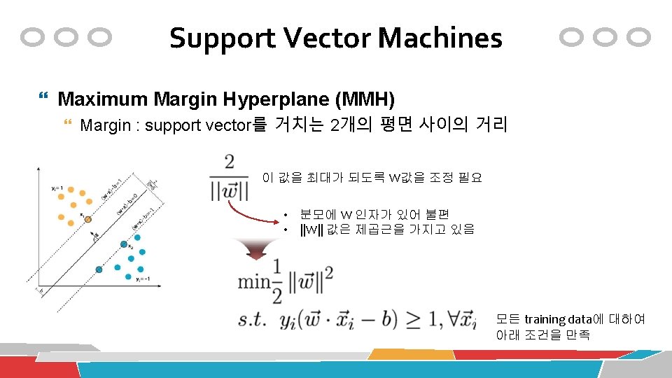
Support Vector Machines Classification with hyperplane 어떤 직선이 가장 좋을까? Maximum Margin Hyperplane (MMH)

Support Vector Machines Hyperplane equation

Support Vector Machines For nonlinearly separable data: soft margin slack variable: creates a soft margin that allows some points to fall on the incorrect side of the margin 분류 조건을 위반하는 데이터는 그 위반 거리만큼의 penalty (cost) 부여

Support Vector Machines For nonlinearly separable data: Kernel function Non-linear relationship -> linear relationship 새로운 feature를 생성

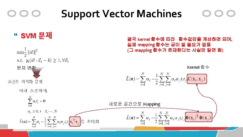
Support Vector Machines 예) Kernel mapping

Support Vector Machines Kernel 함수

Support Vector Machines Kernel 함수 Linear kernel Polynomial kernel Sigmoid kernel Gaussian RBF kernel 많은 경우에 학습 성능이 상대적으로 좋음 마땅한 kernel 함수 의 선택 기준이 없 음 실험을 통해 결정할 수 밖에 없음

Support Vector Machines SVM with non-linear kernels

Support Vector Machines Example – performing OCR with SVMs Image적 특성값

Support Vector Machines Training a model Linear kernel

Support Vector Machines Training a model

Support Vector Machines Evaluating the model

Support Vector Machines Evaluating the model

Support Vector Machines Improving the model Kernel 함수의 교체

Support Vector Machines Improving the model

Unsupervised Learning Association Rule Mining

Apriori algorithm 69

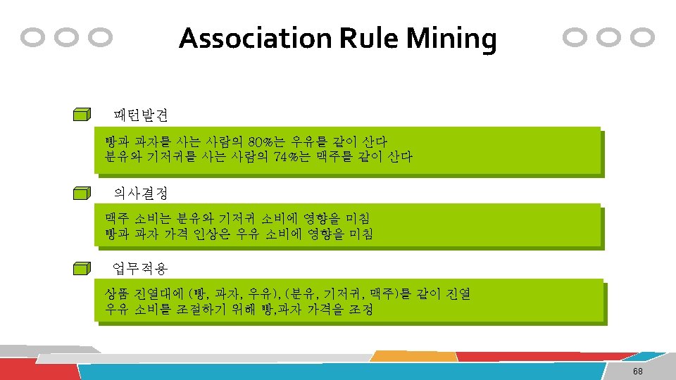
Association Rule Mining Basket (Transaction) data 측정치 (X -> Y) Transaction ID Iterms 1 Chips, Milk 2 Chips, Diaper, Beer, Cornflakes 3 Milk, Diaper, Beer, Pepsi 4 Chips, Milk, Diaper, Beer 5 Chips, Milk, Diaper, pepsi Support (지지도) : 전체 레코드에서 상품 X, Y에 대한 거래를 모두 포함하는 비율 Supp(X, Y) Confidence (신뢰도) : 상품 X를 구매한 거래가 발생했을 경우 그 거래가 상품 Y를 포함하는 조건부 확률 Conf (X->Y) = Supp(X, Y)/Supp(X) Lift (향상도) : 상품 X를 구매한 경우, 그 거래가 상품 Y를 포함하는 경우와 상품 Y가 상품 X에 관계없이 구매된 경우의 비율 => Lift (X->Y)=Supp(X, Y)/(Supp(X)∙Supp(Y)) = Conf(X->Y)/Supp(Y) -> 1이 넘으면 의미 있음 측정치 예 {Milk, Diaper} => Beer : Supp=2/5, Conf=2/3, Lift=(2/3)/(3/5)=1. 1167 70

Association Rule Mining Data Preparation Transaction data

Association Rule Mining Data preparation Non-zero 셀의 비율 9, 835 * 169 = 1, 662, 115 셀 => * 0. 02609146 = 43, 367 물건 구매

Association Rule Mining Data preparation 데이터 내부 관찰 Support 비율

Association Rule Mining Visualizing item support: item frequency plots

Association Rule Mining Visualizing the transaction data: plotting the sparse matrix

Association Rule Mining Training a model

Association Rule Mining Taking subsets of association rules

Association Rule Mining Model visualization

Association Rule Mining Model visualization

Association Rule Mining 일반 데이타베이스에 대한 연관분석 : Adult. UCI 연속형 숫자 속성 컬럼이 있으므로 데이터 가공이 필요 필요없는 속성 제거 # load the data and check it data("Adult. UCI") dim(Adult. UCI) Adult. UCI[1: 2, ] ## remove attributes Adult. UCI[["fnlwgt"]] <- NULL Adult. UCI[["education-num"]] <- NULL

“age”컬럼의 값 들을 변경 Association Rule Mining 구간값을 순서있는 요소로 전환 number -> factor로 변환 일반 데이타베이스에 대한 연관분석 : Adult. UCI 연속형 실수값을 구간값으로 변환 구간 ## map metric attributes Adult. UCI[["age"]] <- ordered(cut(Adult. UCI[["age"]], c(15, 25, 45, 65, 100)), labels = c("Young", "Middle-aged", "Senior", "Old")) Adult. UCI[["hours-per-week"]] <- ordered(cut(Adult. UCI[["hours-per-week"]], c(0, 25, 40, 60, 168)), labels = c("Part-time", "Full-time", "Over-time", "Workaholic")) Adult. UCI[["capital-gain"]] <- ordered(cut(Adult. UCI[["capital-gain"]], c(-Inf, 0, median(Adult. UCI[["capital-gain"]][Adult. UCI[["capital-gain"]]>0]), Inf)), labels = c("None", "Low", "High")) Adult. UCI[["capital-loss"]] <- ordered(cut(Adult. UCI[["capital-loss"]], c(-Inf, 0, median(Adult. UCI[["capital-loss"]][Adult. UCI[["capital-loss"]]>0]), Inf)), labels = c("None", "Low", "High"))

Association Rule Mining 함수형 언어: median 값 찾기 Adult. UCI[["capital-gain"]]>0 “capital-gain” 컬럼의 값들이 0 이상인지 여부 (TRUE/FALSE)를 출력 결국 TRUE/FALSE 값을 가지는 vector를 출력 Adult. UCI[["capital-gain"]] [Adult. UCI[["capital-gain"]]>0] “capital-gain” 컬럼의 값들 중에서 0을 초과한 것만을 추려냄 median( Adult. UCI[["capital-gain"]] [Adult. UCI[["capital-gain"]]>0] ) “capital-gain” 컬럼의 값이 0을 초과한 것들에서 ‘median 값’을 찾아냄

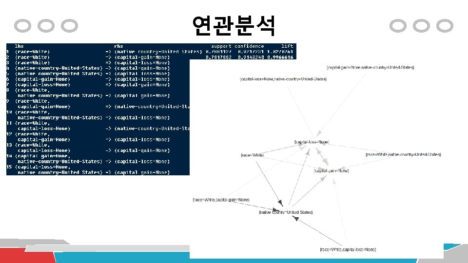
Association Rule Mining {} -> Y 형태 제거 일반 데이타베이스에 대한 연관분석 : Adult. UCI transaction 데이타 포맷으로 변경 Adult <- as(Adult. UCI, "transactions") Apriori 알고리즘으로 연관분석 수행 adult_rules <- apriori(Adult, parameter = list(supp = 0. 7, conf = 0. 9, minlen=2, target = "rules")); inspect(adult_rules) adult_rules. sorted <- sort(adult_rules, by="lift"); inspect(adult_rules. sorted) plot(adult_rules, method = "graph") RHS 부분의 값을 고정하는 경우 adult_rules <- apriori(Adult, parameter = list(supp=0. 35, conf=0. 8, minlen=2, target="rules"), appearance = list(rhs=c(“income=small", “income=large"), default="lhs")) adult_rules. sorted <- sort(adult_rules, by="lift");

Association Rule Mining 중복 규칙이 다수 존재

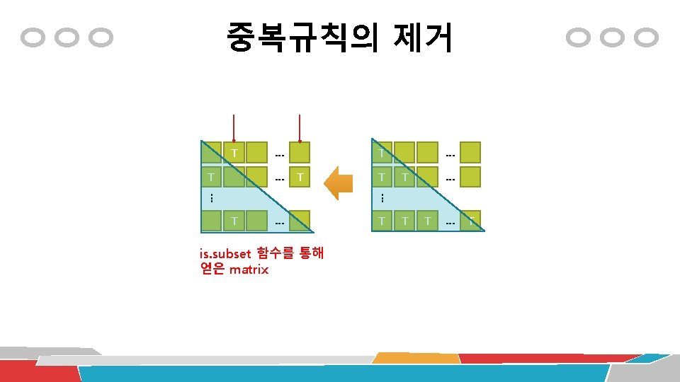
Association Rule Mining 중복 규칙의 제거 집합X의 각 원소(규칙)이 집합Y에 포함 되는 규칙이 있다면 TRUE, 아니면 FALSE를 리턴 # find redundant rules subset. matrix <- is. subset(adult_rules. sorted, adult_rules. sorted) subset. matrix[lower. tri(subset. matrix, diag=T)] <- NA redundant <- col. Sums(subset. matrix, na. rm=T) >= 1 which(redundant) # remove redundant rules TRUE adult_rules. pruned <- adult. rules. sorted[!redundant] inspect(adult_rules. pruned) plot(adult_rules, method = "graph")

Association Rule Mining Exporting the model

Unsupervised Learning Clustering

Clustering 용도 Summarization of large data Understand the large customer data Data organization Manage the large customer data Outlier detection Find unusual customer data Classification/Association Rule Mining의 이전 단계

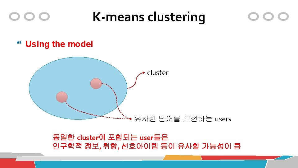
Clustering 용도 Classification/Association Rule Mining의 이전 단계 의미 있는 cluster로부터 class를 도출 Cluster내부에 있는 데이터에 대한 Association Rule Mining을 수행

Clustering 알고리즘의 유형 거리함수(distance function) 기반 계층형 Hierarchical clustering Complete-linkage Single-linkage Centroid-linkage Average-linkage Ward’s method 평면형 Partitional clustering k-means k-medoids 밀도(density) 기반 DBScan

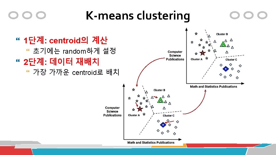
평면형 Clustering: i 단계 k-means : centroid (i+1) 단계 Data Mining Lab. , Univ. of Seoul, Copyright ® 2008 93

K-means clustering

K-means clustering Choosing the appropriate number of clusters one rule of thumb: k = square root of (n / 2) Elbow method

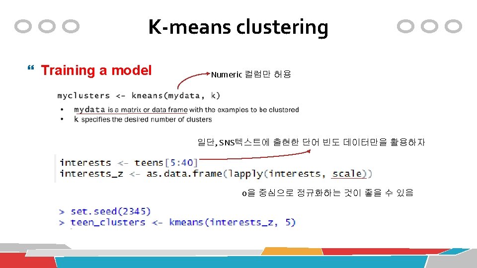
K-means clustering Example: finding teen market segments SNS 메타 정보 SNS 단어출현 정보

K-means clustering Understanding & preparing the data Noise 제거 Noise 의심

K-means clustering Data preparation Missing values가 너무 많다면, 이를 포함한 행을 모두 삭제하는 것은 좋지 않음 => Dummy coding of missing values 확인

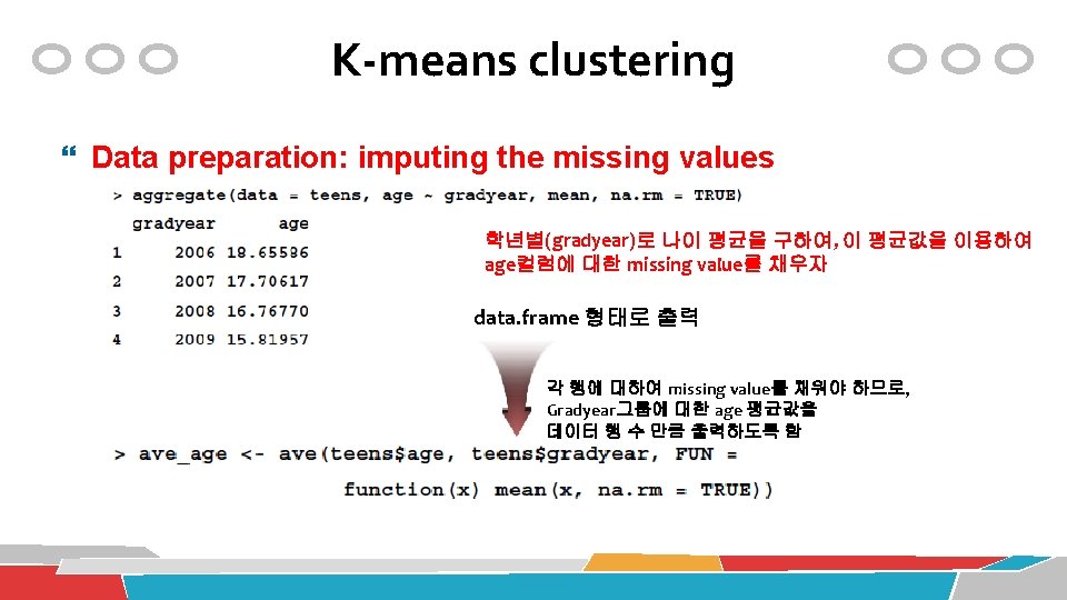
K-means clustering Data preparation: imputing the missing values Imputation: filling in the missing data with a guess as to the true value Missing value를 제거하여 계산 age컬럼의 값을 전체 평균으로 채우는 것은 비합리적 => 다른 컬럼과의 관계를 고려해보자 gradyear 컬럼을 이용: 이 컬럼은 missing value가 없음

K-means clustering Data preparation: imputing the missing values Missing 상태이면, ave_age 값으로 채움 확인

K-means clustering Evaluating the model Z-score 이므로 0보다 크다면 평균 이상을 의미

K-means clustering Evaluating the model

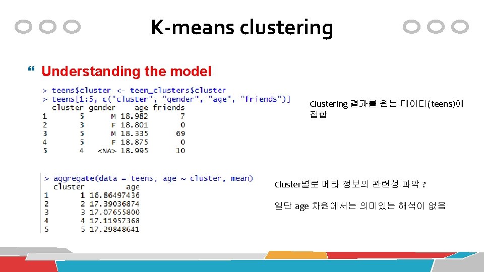
K-means clustering Understanding the model Cluster 2, 5는 female 아닌 사용자가 posting ? SNS에서 여성, 남성이 관심사가 다름을 확인 Clustering 과정에 friends# 를 입력하지 않았지만, Cluster별로 friends# 가 차별화 되고 있음 Clustering: 사용자 behavior를 예측하는 유용한 수단

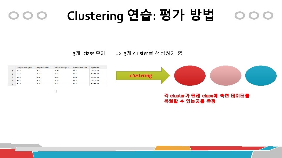
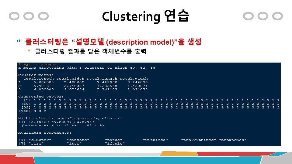
Clustering 연습 K-means 알고리즘의 활용 data(iris) library(stats) myiris <-iris myiris$Species <-NULL # Species 컬럼 제거 myiris. kmeans <- kmeans(myiris, centers=3) myiris. kmeans <- kmeans(myiris, 3) # 위와 동일한 표현 3개의 cluster를 생성

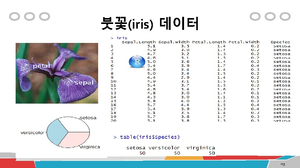
Iris Data

붓꽃(iris) 데이터 virginica versicolor 어떤 종류인가? ? setosa 111

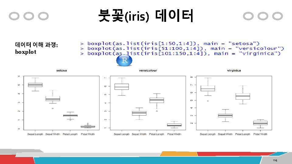
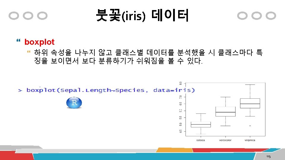
붓꽃(iris) 데이터 붓꽃데이터 3가지 종류(class): setosa, versicolor, virginica 4가지 주요 속성값을 토대로 class를 분류? 꽃받침길이(Sepal. Length) 꽃받침폭(Sepal. width) 꽃잎길이(Petal. Length) 꽃잎폭(Petal. Width) 112

붓꽃(iris) 데이터 pairs(iris[1: 4], main = "Anderson's Iris Data -- 3 species", pch = 21, bg = c("red", "green 3", "blue")[unclass(iris$Species)]) Scatter Plot 2개의 속성간의 관계를 파악 116

Clustering 연습 K-means 알고리즘의 평가: 기존 class분류결과와 비교 table(iris$Species, myiris. kmeans$cluster) conf. mat <- table(iris$Species, myiris. kmeans$cluster) (accuracy <- sum(diag(conf. mat))/sum(conf. mat) * 100) new. mat <- data. frame("c 1"=conf. mat[, 1], "c 3"=conf. mat[, 3], "c 2"=conf. mat[, 2]) new. mat <- as. matrix(new. mat) (accuracy <- sum(diag(new. mat))/sum(new. mat) * 100) as. OOO 형태의 함수 Cluster 배치 변경 # 사실은, 아래와 같이 간단하게 > new. mat <- conf. mat[, c(1, 3, 2)]

Clustering 연습 K-means 모델의 시각화 클러스터 번호를 col속성에 할당 데이터 항목별로 color값을 할당 plot(myiris[c("Sepal. Length", table(iris$Species, myiris. kmeans$cluster) "Sepal. Width")], col=myiris. kmeans$cluster) conf. mat <- table(iris$Species, myiris. kmeans$cluster) points(myiris. kmeans$centers[, c("Sepal. Length", "Sepal. Width")], col=1: 3, pch=“*”, cex=5)

Clustering 연습 K-means 모델의 해석 myiris. kmeans$centers # 각 cluster의 중심값을 출력 ave <- 0 for(i in 1: ncol(myiris)) ave[i]<- sum(myiris. kmeans$centers[, i])/nrow(myiris. kmeans$centers) ave # 출력

Clustering 연습: Iris 데이터 K-means 모델 평가 conf. mat <- table(iris$Species, km$cluster) (accuracy <- sum(diag(conf. mat))/sum(conf. mat) * 100) Cluster Class

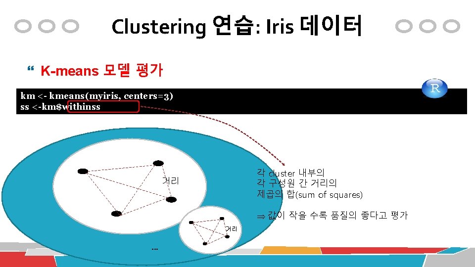
Clustering 연습: Iris 데이터 K-means 모델의 평가 ss <-0 for(i in 2: 15) ss[i] <- sum(kmeans(myiris, centers=i)$withinss) plot(2: 15, ss, type="b", xlab="클러스터 개수", ylab="각 클러스터 SSE의 합")

Clustering 연습: Iris 데이터 K-means 알고리즘의 활용: cluster 품질평가 ss <-0 for(i in 1: 15) ss[i] <- sum(kmeans(mywine, centers=i)$withinss) plot(1: 15, ss, type="b", xlab="클러스터 개수", ylab="각 클러스터 SS의 합")

Clustering 연습 K-medoids 알고리즘의 활용 library(cluster) myiris. pam <- pam(myiris, 3) table (myiris. pam$clustering, iris$Species) VS. K-means 모델 K-medoids 모델 Outlier에 강함 ! why? outlier에 약함

계층형 clustering 0 step a 1 step 2 step 3 step Bottom-up (agglomerative) ab b abcde c cde e de d 4 step 3 step 2 step 1 step 0 step Top-down (divisive) Data Mining Lab. , Univ. of Seoul, Copyright ® 2008 127

Hierarchical Agglomerative Clustering (HAC) 5가지 유형 Simple linkage Complete linkage Average linkage Centroid linkage Ward’s method Sum of Square Error (SSE) 계산

HAC: distance functions Euclidean 거리함수 Manhattan 거리함수 Minkowski 거리함수 Canberra 거리함수

HAC clustering HAC 알고리즘의 활용: single linkage table(iris$Species, cls$cluster) sim_eu <- dist(myiris, method="euclidean") conf. mat <- table(iris$Species, cls$cluster) dendrogram <-hclust(sim_eu^2, method=“single”) plot(dendrogram) cluster <- cutree(dendrogram, k=3) table(iris$Species, cluster)

HAC clustering sim_eu <- dist(myiris, method="euclidean") "euclidean", "manhattan", "canberra", "minkowski" dendrogram <-hclust(sim_eu^2, method=“single”) "ward. D 2", "single", "complete", "average" , "median“, "centroid"

HAC clustering HAC 모델의 시각화: dendrogram Cutting line에 따라 cluster 개수가 결정

HAC clustering small iris 데이터의 군집분석 iris. num <- dim(iris)[1] # nrow(iris) 와 동일 idx <-sample(1: iris. num, 50) smalliris <- iris[idx, ] smalliris$Species <-NULL sim <- dist(smalliris) den <- hclust(sim^2, method="single") plot(den, hang= -1, labels=iris$Species[idx])

HAC clustering �HAC 모델의 시각화: dendrogram plot(den, hang= -1) plot(den, hang= -1, labels=iris$Species[idx])

HAC clustering �HAC 알고리즘의 활용: average linkage sim_eu <- dist(myiris, method="euclidean") dendrogram <-hclust(sim_eu^2, method=“average”) plot(dendrogram) cluster <- cutree(dendrogram, k=3) conf. mat <- table(iris$Species, cluster) HAC 알고리즘의 활용: complete linkage (accuracy <- sum(diag(conf. mat))/sum(conf. mat) * 100)

HAC clustering �HAC 알고리즘의 활용: complete linkage sim_eu <- dist(myiris, method="euclidean") table(iris$Species, cls$cluster) dendrogram <-hclust(sim_eu^2, method=“complete”) conf. mat <- table(iris$Species, cls$cluster) plot(dendrogram) cluster <- cutree(dendrogram, k=3) conf. mat <- table(iris$Species, cluster) (accuracy <- sum(diag(conf. mat))/sum(conf. mat) * 100) HAC 알고리즘의 활용: complete linkage new. mat <- data. frame("c 1"=conf. mat[, 1], "c 3"=conf. mat[, 3], "c 2"=conf. mat[, 2]) new. mat <- as. matrix(new. mat) (accuracy <- sum(diag(new. mat))/sum(new. mat) * 100) Cluster 배치 변경

HAC clustering �HAC 알고리즘의 활용: Ward’s method sim_eu <- dist(myiris, method="euclidean") dendrogram <-hclust(sim_eu^2, method=“ward. D”) plot(dendrogram) cluster <- cutree(dendrogram, k=3) conf. mat <- table(iris$Species, cluster) HAC 알고리즘의 활용: complete linkage (accuracy <- sum(diag(conf. mat))/sum(conf. mat) * 100)

HAC clustering �HAC 알고리즘의 활용: centroid linkage sim_eu <- dist(myiris, method="euclidean") dendrogram <-hclust(sim_eu^2, method=“centroid”) plot(dendrogram) cluster <- cutree(dendrogram, k=3) conf. mat <- table(iris$Species, cluster) HAC 알고리즘의 활용: complete linkage (accuracy <- sum(diag(conf. mat))/sum(conf. mat) * 100)

HAC clustering �HAC 알고리즘의 활용: centroid linkage 거리함수 변경 sim_mi <- dist(myiris, method="minkowski") dendrogram <-hclust(sim_mi^2, method=“centroid”) plot(dendrogram) HAC 알고리즘의 활용: complete linkage cluster <- cutree(dendrogram, k=3) conf. mat <- table(iris$Species, cluster) (accuracy <- sum(diag(conf. mat))/sum(conf. mat) * 100)

Density-based clustering DBSCAN: Cluster를 “density-connected set”으로 정의 density: 정해진 반경( )내에 데이터의 개수 Data Mining Lab. , Univ. of Seoul, Copyright ® 2008

Density-based clustering 알고리즘의 활용 library(fpc) myiris <- iris[-5] myiris. ds <- dbscan(myiris, eps=0. 42, Min. Pts=5) table(myiris. ds$cluster, iris$Species)

Density-based clustering: Iris 데이터 Density-based clustering 모델의 평가 plot(myiris. ds, myiris)

Density-based clustering: Iris 데이터 Density-based clustering 모델의 평가 plot(myiris. ds, myiris[c(1, 4)])

Density-based clustering: Iris 데이터 Density-based clustering 모델의 평가 plotcluster(myiris, myiris. ds$cluster) # projection

Performance Evaluation

Measuring performance for classification confusion matrix

Measuring performance for classification confusion matrix

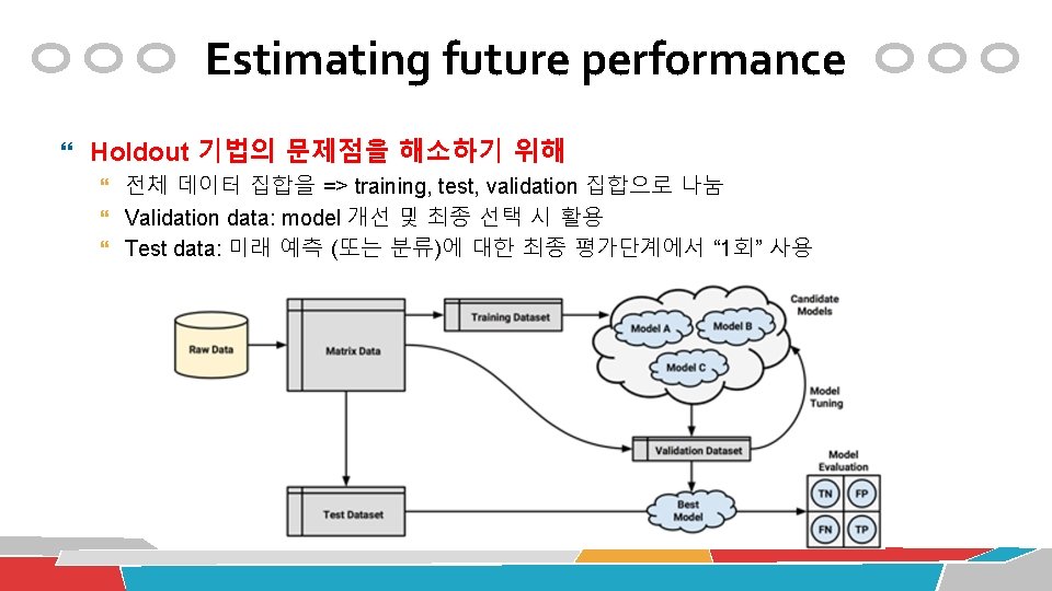
Estimating future performance Holdout method 일반적으로, 전체데이터의 2/3 => training, 1/3 => testing holdout을 여러 번 반복하여 best model을 취함 test data는 model 생성에 영향을 미치지 않아야 함 하지만, random하게 잡은 training data에 대하여 다수의 model을 생성한 후, test data에 대하여 best model을 찾는 것이어서, hold-out 기법에서의 test performance는 공정하지 않음

Estimating future performance Validation 집합을 포함한 일반적 비율 (training, test, validation) = (50%, 25%)

Estimating future performance 최종 모델 선택하기까지 단 순 Holdout 기법은 편향된 model을 생성할 수 있 음 Repeated Holdout (k-fold cross validation) caret 패지지의 create. Folds() 함수 활용 1 2 3 4 5 6 7 8 9 10

Estimating future performance C 5. 0 decision trees에 대한 k-folds CV 수행 첫번째 fold를 test data로 설정하여, 모델 평가

Estimating future performance lapply()을 사용, C 5. 0 decision trees에 대한 k-folds CV 자동화

Automated Parameter Tuning

Automated Parameter Tuning train() 함수의 활용 임의의 machine learning 알고리즘을 구동시켜줌 train() 함수의 아래의 요소를 지정해줘야 함 machine learning algorithm model parameters model evaluation criteria

Automated Parameter Tuning train() 함수의 활용: learning algorithm & model parameters

Automated Parameter Tuning Creating a simple tuned model http: //topepo. github. io/caret/bytag. html

Automated Parameter Tuning Bootstrap Sampling Training data

Automated Parameter Tuning Testing and Evaluation

Automated Parameter Tuning Customizing the tuning process train. Control() 함수 Train() 함수를 guide하는 configuration 집합을 생성 Resampling 전략, best model 선택 방법 등을 명시

Automated Parameter Tuning Customizing the tuning process Grid 설정 Grid: learning parameter의 조합

Automated Parameter Tuning Customizing the tuning process Training a model Regression: "RMSE“, "Rsquared“ Classification: "Accuracy“, "Kappa"

Meta-Learning

Meta Learning 임의의 machine learning 알고리즘에 대하여 포괄적으로 적용할 수 있는 기술 Ensemble § Bagging § Boosting § Random Forests Semi-Supervised Learning § EM Active Learning § Selective Sampling 164

Ensemble Methods • Overfitting 가능성 줄임 • Model의 bias-variance 줄임 • 분산처리가 용이

Bagging (Bootstrap Aggregation) Sampling with replacement 각 bootstrap sample 집합에 대하여 하나의 (weak) model을 생성 보통 25개의 model을 생성 test data 각각에 대하여 voting을 통해 class 결정 Daniel Spohn Youngstown State University

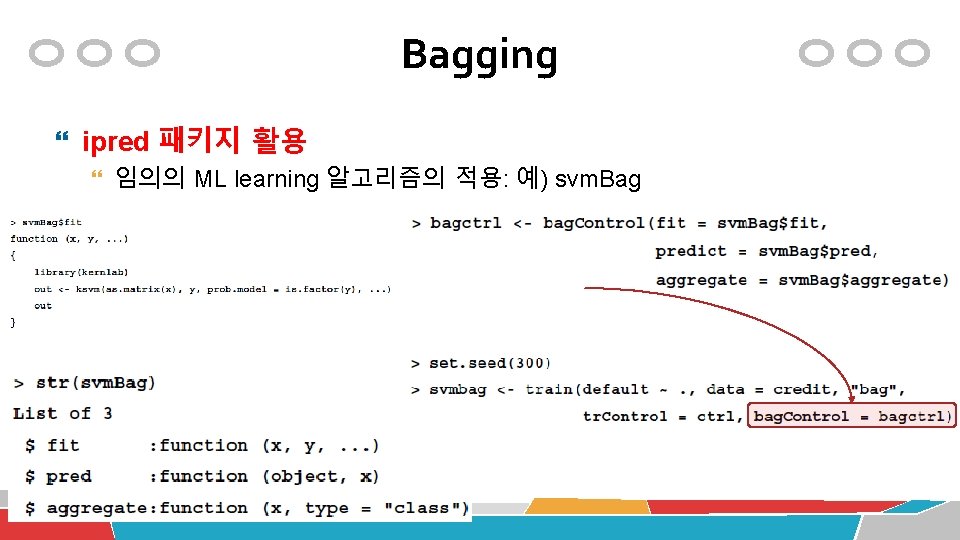
Bagging ipred 패키지 활용 decision trees에 대한 bagging * train() 함수의 활용 10 -folds CV ipred패키지의 bagged tree 기법

Ada. Boosting (Adaptive Boosting) Base (weak) classifiers: C 1, C 2, …, CT Error rate: Importance of a classifier:

Ada. Boosting (Adaptive Boosting) Weight 갱신: Classification: 각 base classifier Cj에 j만큼의 classification weight 부여

Ada. Boosting (Adaptive Boosting)

Ada. Boosting (Adaptive Boosting) Ada. Boost. M 1: tree-based implementation of Ada. Boost for classification

Random Forests Decision Trees-based Ensemble n개의 Bootstrap samples 각 bootstrap sample에서 random하게 m개의 컬럼(독립) 변수 선택하여 tree 생성 Pruning 없음 Classification을 위해서 일반적 Bagging 처럼 voting함

Random Forests Training a model

Random Forests Evaluating the model

EM Algorithm Training data의 부족 문제 Training data의 구축은 시간, 비용이 많이 소요되는 작업 EM (Expectation-Maximization) algorithm 적은 양의 labeled training data를 가지고 unlabeled training data를 반복 적으로 labeling 즉, labeled data를 중심으로 unlabeled training data를 clustering 177

EM Algorithm with Naïve Bayes Classification model of NB classifiers - Class prior estimate - Word probability estimate Class prior estimate Word probability estimate 178

EM Algorithm with Naïve Bayes Unlabeled documents Classifier Classified documents E-step Initial Training Set M-step Learner 179

EM Algorithm upclass 패키지 활용: Iris 데이터

EM Algorithm Data Preparation 전체 data 중에서 1/5 비율의 training data 생성

EM Algorithm Training a model using Labeled and Unlabeled data EM 과정 수행

EM Algorithm Evaluating the model

EM Algorithm Decision Tree와의 비교

Active Learning Pool-based Active Learning Training을 목적으로 labeling할 데이터를 쌓아두고, 이 중에서 learning에 도움이 되는 데이터만 을 선택하여 labeling

Active Learning Uncertainty-based Active Learning 분류결정 boundary 근처에 있는 데이터를 Labeling하는 것이 model 개선에 큰 도움이 됨

Active Learning Uncertainty-based Active Learning Classification Uncertainty의 정의 Xd를 주어진 model에 근거하여 class 집합 C={c 1, c 2, …, c|c|}의 원소 중의 하나로 분 류한다고 가정할 때, 각 class에 속할 확률이 P = {p 1, p 2, …, p|c|}. Entropy 기반 classification uncertainty