207 4 5 Undetermined Coefficients Annihilator Approach For

 annihilator: D")
2 = D 2 − 4 D + 4 註:當")


 = g 1(x) + g 2(x) + …… +")

 annihilator: D 3 annihilator: D − 5 annihilator:")


 Step 1: Complementary function")

 Step 1: Complementary function From auxiliary function, m")

 所以要先算 complementary function,再算 particular solution (2) 若有兩個以上的 annihilator,選其中較簡單的即可")


 相比較")

 Step 1: solution of Step")

 Note: (a) 的算法 (b) Interval (0, /6) 改為(0,")


![4 -7 -3 For the 2 nd Order Case auxiliary function: roots [Case 1]:](https://slidetodoc.com/presentation_image_h/c57a18ed895fe54de1c0355289752275/image-35.jpg "4 -7 -3 For the 2 nd Order Case auxiliary function: roots [Case 1]:")
![242 [Case 2]: m 1 = m 2 Use the method of reduction of](https://slidetodoc.com/presentation_image_h/c57a18ed895fe54de1c0355289752275/image-36.jpg "242 [Case 2]: m 1 = m 2 Use the method of reduction of")
 is a solution of a homogeneous DE then c y")
![244 [Case 3]: m 1 m 2 and m 1, m 2 are the](https://slidetodoc.com/presentation_image_h/c57a18ed895fe54de1c0355289752275/image-38.jpg "244 [Case 3]: m 1 m 2 and m 1, m 2 are the")
 Example 2 (text page 164) Example 3 (text")

 若 auxiliary function 在 m 0 的地方只有一個根 是 associated homogeneous equation 的其中一個解")
 若 auxiliary function 在 + j 和 − j 的地方各有一個根 (未出現重根) 是")
 auxiliary function 249")

 Step 1 solution of the associated homogeneous equation auxiliary")

 Set x = et, t = ln x (chain")
 Note 1: 以此類推 Note 2: 簡化計算的小技巧:結合兩種解 nonhomogeneous")
 本節公式記憶的方法: 把 Section 4 -3 的 ex 改成 x,x")
 numerical approach (Section 4 -9 -3) (2) using")


 名詞一 被稱作 input 或 deriving function 或 forcing function 被稱作 output")
 名詞二 對一個 2 nd order linear DE with constant coefficients auxiliary function")

 (m")
 E(t) 有的時候可用”guess” 的方法來解 (2) E(t) 用 variation of parameters 的方法一定解得出來(但較耗時 )")
 = E 0 where E 0 is some constant (m")
 (m 1 =")
 when t Particular solution")
 = E 0 where E 0 is some constant When R =")
 = 1, L = 0. 25, C = 0. 01")


 Express the Solution by")

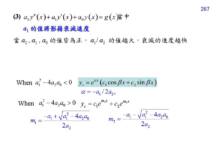
 Express the Solution by Hyperbolic Functions 當 a 1 = 0 且")

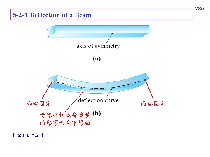
 牛頓運動定律 (2) 彈簧運動 (subsection 5 -1 -1~5 -1 -3)")

: bending moment at the point x w(x): load per unit length EI:")
 (a) embedded at")


 T y'(x + x) = xy 2 boundary condition: y(0) = 0,")

")
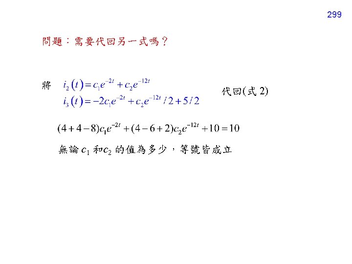
 Step 1 ……. . (式 2) Step 2 -1")
 − (D+10) (式 2) Step 3 -2")
 Example 3 (text")
 (式 2) Step 1 Step 2 -1 (式")
 (D+1) − (式 2) (D− 4) Step 3 -2")


 (Step 1) 問題: u 要用什麼方法解? (Step 2) (Step")

 (Step 1) Set (Step 2) (Step 3)")

 : 代回 Taylor series 319")


 鍾擺的例子 (text pages 209,")
")
 Cauchy-Euler equation 缺乏應用 (2) 許多情形還是只能用 Numerical Method 來解")
 Linear DE Complementary Function 3 大解法 (1) Reduction")
 Cauchy-Euler Equation (Section 4 -7) 適用情形: 336")
 Linear DE Particular solution 3 大解法 (1) Guess (Section 4 -4) (熟悉講義 page")
 Variation of parameters (Section 4 -6) Wk : replace the kth column of")
 For Cauchy-Euler Equation (Section 4 -7) 可採用二種方法 (1) 先用 解 complementary function 再用")
 Combination of Linear DEs (Section 4 -8) 方法: Step 1: 將 變成 Dn")
 Nonlinear DE 的3大解法 (Section 4 -9) (1) Reduction of Order (1 -1) Set")
 Taylor Series 適用情形: (3) Numerical Method 適用情形:")

- Slides: 137
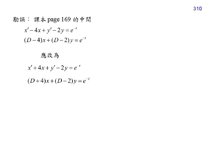
207 4 -5 Undetermined Coefficients – Annihilator Approach For a linear DE: Annihilator Operator: 能夠「殲滅」 g(x) 的 operator 4 -5 -1 方法適用條件 (1) Linear, (2) Constant coefficients (3) g(x), g'''(x), g(4)(x), g(5)(x), ………contain finite number of terms.
208 4 -5 -2 Find the Annihilator Example 1: (text page 151) annihilator: D 4 annihilator: D + 3
209 annihilator: (D − 2)2 = D 2 − 4 D + 4 註:當 coefficient 為 constants 時,function of D 的計算方式 和 function of x 的計算方式相同 (x − 2)2 = x 2 − 4 x + 4 (D − 2)2 = D 2 − 4 D + 4
210 General rule 1: If then the annihilator is 注意: annihilator 和 a 0, a 1, …… , an 無關 只和 , n 有關
General rule 2: If b 1 0 or b 2 0 then the annihilator is Example 2: (text page 151) annihilator Example 5: (text page 154) annihilator Example 6: (text page 155) annihilator 211
General rule 3: If g(x) = g 1(x) + g 2(x) + …… + gk(x) Lh[gh(x)] = 0 but Lh[gm(x)] 0 if m h, then the annihilator of g(x) is the product of Lh (h = 1 ~ k) Proof: (因為 L 1, L 2 為 linear DE with constant coefficient, L 1 L 2 = L 2 L 1 ) 212
213 Similarly, : : Therefore,
214 Example 7 (text page 155) annihilator: D 3 annihilator: D − 5 annihilator: (D − 2)3 annihilator of g(x): D 3 (D − 2)3 (D − 5)
215 4 -5 -3 Using the Annihilator to Find the Particular Solution Step 2 -1 Find the annihilator L 1 of g(x) Step 2 -2 如果原來的 linear & constant coefficient DE 是 那麼將 DE 變成如下的型態: (homogeneous linear & constant coefficient DE) 註: If then
216 Step 2 -3 Use the method in Section 4 -3 to find the solution of Step 2 -4 Find the particular solution. The particular solution yp is a solution of but not a solution of (Proof): Since Moreover, Step 2 -5 Solve the unknowns , if g(x) 0, should be nonzero. .
217 solutions of particular solution yp solutions of
218 4 -5 -4 Examples Example 3 (text page 153) Step 1: Complementary function (solution of the associated homogeneous function) Step 2 -1: Annihilation: D 3 Step 2 -2: Step 2 -3: auxiliary function roots: m 1 = m 2 = m 3 = 0, m 4 = − 1, m 5 = − 2 Solution for :
Step 2 -4: particular solution Step 2 -5: Step 3: 219
220 Example 4 (text page 154) Step 1: Complementary function From auxiliary function, m 2 − 3 m = 0, roots: 0, 3 Step 2 -1: Find the annihilator D− 3 annihilate but cannot annihilate (D 2 + 1) annihilate but cannot annihilate (D − 3)(D 2 + 1) is the annihilator of Step 2 -2:
Step 2 -3: auxiliary function: solution of 代回原式 並比較係數 Step 3: general solution 易犯錯的地方 : Step 2 -4: particular solution Step 2 -5: 221
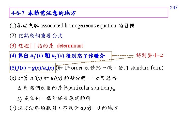
222 4 -5 -5 本節要注意的地方 (1) 所以要先算 complementary function,再算 particular solution (2) 若有兩個以上的 annihilator,選其中較簡單的即可 (3) 計算 auxiliary function 時有時容易犯錯 (4) 的解和 的解不一樣。 (5) 這方法,只適用於 constant coefficient linear DE (因為,還需借助 auxiliary function)
223 The thing that can be done by the annihilator approach can always be done by the “guessing” method in Section 4 -4, too.
224 4 -6 Variation of Parameters 4 -6 -1 方法的限制 The method can solve the particular solution for any linear DE (1) May not have constant coefficients (2) g(x) may not be of the special forms
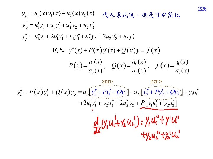
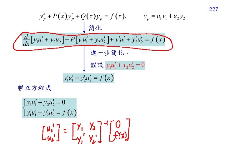
225 4 -6 -2 Case of the 2 nd order linear DE associated homogeneous equation: Suppose that the solution of the associated homogeneous equation is Then the particular solution is assumed as:
228 where | |: determinant 可以和 1 st order case (page 56) 相比較
4 -6 -3 Process for the 2 nd Order Case Step 2 -1 變成 standard form Step 2 -2 Step 2 -3 Step 2 -4 Step 2 -5 229
4 -6 -4 Examples Example 1 (text page 159) Step 1: solution of Step 2 -2: Step 2 -3: 230
Step 2 -4: Step 2 -5: Step 3: 231
232 Example 2 (text page 159) Note: (a) 的算法 (b) Interval (0, /6) 改為(0, /3) Example 3 (text page 160) Note: 沒有 analytic 的解 所以直接表示成 (複習 page 43)
233 4 -6 -5 Case of the Higher Order Linear DE Solution of the associated homogeneous equation: The particular solution is assumed as:
234
235 Wk: replace the kth column of W by For example, when n = 3,
4 -6 -6 Process of the Higher Order Case Step 2 -1 變成 standard form Step 2 -2 Calculate W, W 1, W 2, …. , Wn (see page 234) Step 2 -3 Step 2 -4 Step 2 -5 ……… ……. 236
238 4 -7 Cauchy-Euler Equation 4 -7 -1 解法限制條件 not constant coefficients k but the coefficients of y(k)(x) have the form of ak is some constant associated homogeneous equation particular solution
4 -7 -2 解法 Associated homogeneous equation of the Cauchy-Euler equation Guess the solution as y(x) = xm , then 239
240 auxiliary function 比較: 和 constant coefficient 時有何不同? 規則:把 變成
4 -7 -3 For the 2 nd Order Case auxiliary function: roots [Case 1]: m 1 m 2 and m 1, m 2 are real two independent solution of the homogeneous part: 241
242 [Case 2]: m 1 = m 2 Use the method of reduction of order Note 1: 原式 Note 2: 此時
243 If y 2(x) is a solution of a homogeneous DE then c y 2(x) is also a solution of the homogeneous DE If we constrain that x > 0, then
244 [Case 3]: m 1 m 2 and m 1, m 2 are the form of two independent solution of the homogeneous part: 同理
245 Example 1 (text page 164) Example 2 (text page 164) Example 3 (text page 165)
246 4 -7 -4 For the Higher Order Case Process: auxiliary function roots independent solutions Step 1 -1 Step 1 -2 solution of the associated Step 1 -3 homogeneous equation
247 (1) 若 auxiliary function 在 m 0 的地方只有一個根 是 associated homogeneous equation 的其中一個解 (2) 若 auxiliary function 在 m 0 的地方有 k 個重根 皆為 associated homogeneous equation 的解
248 (3) 若 auxiliary function 在 + j 和 − j 的地方各有一個根 (未出現重根) 是 associated homogeneous equation 的其中二個解 (4) 若 auxiliary function 在 + j 和 − j 的地方皆有 k 個重根 是 associated homogeneous equation 的其中 2 k 個解
Example 4 (text page 166) auxiliary function 249
250 4 -7 -5 Nonhomogeneous Case To solve the nonhomogeneous Cauchy-Euler equation: Method 1: (See Example 5) (1) Find the complementary function (general solutions of the associated homogeneous equation) from the rules on pages 241 -248. (2) Use the method in Sec. 4 -6 (Variation of Parameters) to find the particular solution. (3) Solution = complementary function + particular solution Method 2: See Example 6,重要 Set x = et, t = ln x
Example 5 (text page 166) Step 1 solution of the associated homogeneous equation auxiliary function Step 2 -2 Particular solution Step 2 -3 251
252 Step 2 -4 Step 2 -5 Step 3
Example 6 (text page 167) Set x = et, t = ln x (chain rule) Therefore, the original equation is changed into 253
254 (別忘了 t = ln x 要代回來) Note 1: 以此類推 Note 2: 簡化計算的小技巧:結合兩種解 nonhomogeneous Cauchy. Euler equation 的長處
4 -7 -6 本節要注意的地方 (1) 本節公式記憶的方法: 把 Section 4 -3 的 ex 改成 x,x 改成 ln(x) 把 auxiliary function 的 mn 改成 (2) 如何解 particular solution? Variation of Parameters 的方法 (3) 解的範圍將不包括 x = 0 的地方 (Why? ) 255
256 還有很多 linear DE 沒有辦法解,怎麼辦 (1) numerical approach (Section 4 -9 -3) (2) using special function (Chap. 6) (3) Laplace transform and Fourier transform (Chaps. 7, 11, 14) (4) 查表 (table lookup)
258 Exercise for practice Section 4 -4 5, 6, 14, 17, 18, 24, 26, 33, 39, 42 Section 4 -5 2, 7, 13, 18, 31, 45, 69, 70 Section 4 -6 4, 5, 8, 13, 14, 18, 21, 24, 25, 28 Section 4 -7 11, 17, 18, 20, 21, 32, 34, 36, 37 Review 4 2, 13, 14, 17, 19, 20, 23, 24, 27, 32 得出 implicit solution 即可 Homework 2 (Due: 28 th Oct. ) (1) Sec. 2 -4 8 (2) Sec. 2 -5 9 (3) Sec. 2 -5 15 (4) Review 2 18 (5) Sec. 4 -2 5 (6) Sec. 4 -2 12 (7) Sec. 4 -3 25 (8) Sec. 4 -4 22 (9) Sec. 4 -5 39 (10) Sec. 4 -6 11
259 Chapter 5 Modeling with Higher Order Differential Equations Chapter 4 的應用題 自然界,有不少的系統可以用 linear DE 來表示 其中有不少的系統可以進一步簡化成 linear DE with constant coefficients
260 5 -1 Linear Models: Initial Value Problem 位置:x, 速度: v: 速度, v: 磨擦力 加速度
261 5 -1 -1 ~ 5 -1 -3 Spring / Mass Systems 彈力 F Figure 5. 1. 1 Spring/mass system
262 Solution: Figure 5. 1. 4
263 彈力 F Figure 5. 1. 5 摩擦力
265 需要注意的概念 (1) 名詞一 被稱作 input 或 deriving function 或 forcing function 被稱作 output 或 response
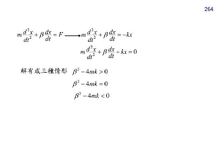
266 (2) 名詞二 對一個 2 nd order linear DE with constant coefficients auxiliary function 當 時,稱作 overdamped 當 時,稱作 critical damped 當 時,稱作 underdamped 當 , a 1 = 0 時,稱作 undamped
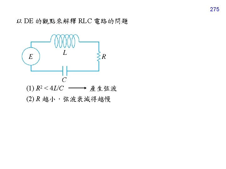
268 5 -1 -4 RLC circuit inductance 的電壓 capacitor 的電壓 resistor 的電壓 using 一定可以解
269 auxiliary function roots: Case 1: R 2 4 L/C > 0 (overdamped) (m 1 m 2, m 1, m 2 are real) 註:由於 R, L, C 的值都是正的, 所以 m 1, m 2 都是負的 when t 必定可以滿足
Particular solution (1) E(t) 有的時候可用”guess” 的方法來解 (2) E(t) 用 variation of parameters 的方法一定解得出來(但較耗時 ) 270
271 Specially, when E(t) = E 0 where E 0 is some constant (m 1 m 2 = 1/LC)
272 Case 2: R 2 4 L/C = 0 (critically damped) (m 1 = m 2 = R/2 L) when t Particular solution When E(t) = E 0 ,
Case 3: R 2 4 L/C < 0 273 (underdamped) when t Particular solution General solution
When E(t) = E 0 where E 0 is some constant When R = 0 , then = 0 When R = 0 , E(t) = E 0 274
276 例子 E(t) = 1, L = 0. 25, C = 0. 01
277 R = 100 R = 25 R = 10
278 R=5 R = 1. 5 R = 0. 2
5 -1 -5 Express the Solutions by Other Forms (1) Express the Solution by the Form of Amplitude and Phase 當 時,solution 為 Solution 可改寫成 279
280 damped amplitude damped frequency phase angle
281 (2) Express the Solution by Hyperbolic Functions 當 a 1 = 0 且 a 2 > 0, a 0 < 0 (或 a 0 > 0, a 2 < 0)
283 5 -2 Linear Models: Boundary-Value Problem Section 5 -2 的問題,和 Section 5 -1 類似 (都是 Linear DE) 只是將 initial value problems 變成 boundary value problems 複習: 將 IVP 改成 boundary value problems, 對 solution 有什麼影響?
Section 5 -1 的例子 (1) 牛頓運動定律 (2) 彈簧運動 (subsection 5 -1 -1~5 -1 -3) (3) RLC Circuit (subsection 5 -1 -4) Section 5 -2 的例子 (1) 樑彎曲 (a) 橫放 (subsection 5 -2 -1) (b) 上方施力 (subsection 5 -2 -2) (2) 跳繩 (subsection 5 -2 -3) 284
y-axis 嵌入 embedded 懸掛 hinged Figure 5. 2. 2 286 embedded x-axis 非固定 free hinged
287 M(x): bending moment at the point x w(x): load per unit length EI: flexural rigidity (some constant)
288 Boundary values for the 3 cases (plotted on page 286) (a) embedded at x 0: y(x 0) = 0, y'(x 0) = 0 (b) free at x 0: y''(x 0) = 0, y'''(x 0) = 0 (c) simply supported or hinged: y(x 0) = 0, y''(x 0) = 0 Case of the 2 nd example on page 286 y(0) = 0, y''(L) = 0, y'''(L) = 0
5 -2 -2 Bucking of a Thin Vertical Column P: 在上 方施力 Figure 5. 2. 4 289
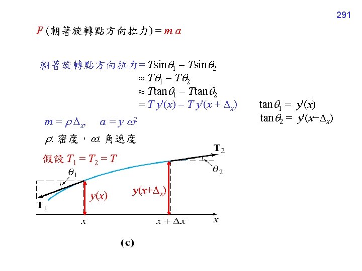
290 5 -2 -3 Rotating String y-axis 繞著軸旋轉 x-axis 假設 T 1 = T 2 = T
T y'(x) T y'(x + x) = xy 2 boundary condition: y(0) = 0, y(L) = 0 292
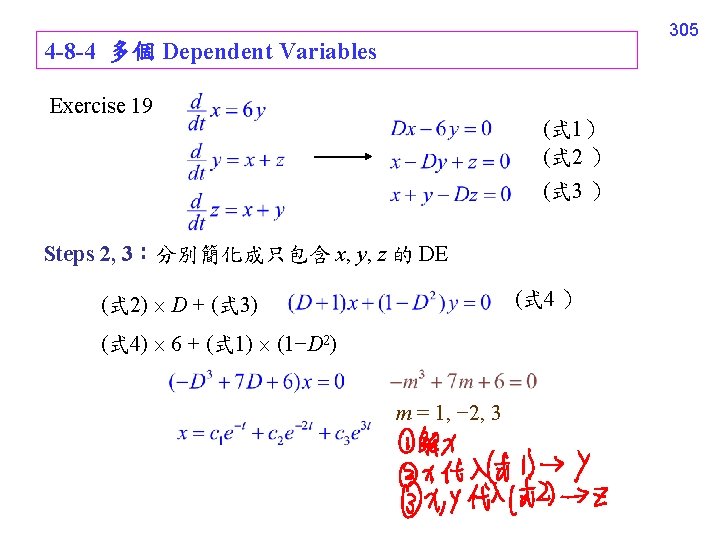
293 4 -8 Solving Systems of Linear Equations by Elimination 4 -8 -1 方法適用的情形和限制 處理有 2 個以上 dependent variables 的問題 例如:Section 3 -3 電路學上 “並聯” 的例子 限制:必需是 linear and constant coefficients
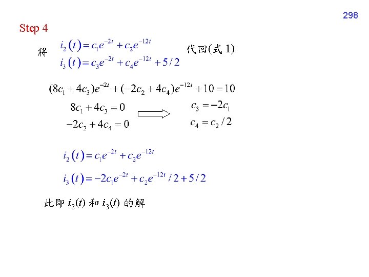
295 4 -8 -3 範例 Figure 3. 3. 4 的例子 (See Pages 94, 95) 令 L 1 = L 2 = 1, R 1 = 6, R 2 = 4, E(t) = 10 求解
296 ……. . (式 1) Step 1 ……. . (式 2) Step 2 -1 (D + 4) (式 1) − 4 (式 2) Note: Step 3 -1 auxiliary function: roots
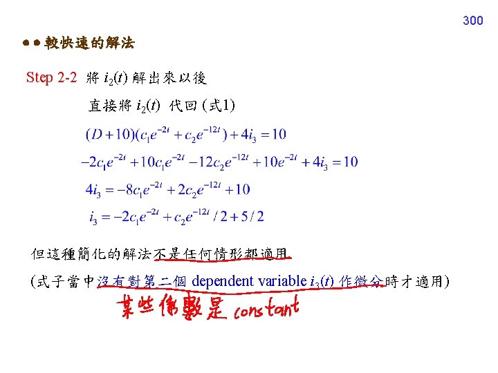
297 Step 2 -2 4 (式 1) − (D+10) (式 2) Step 3 -2 auxiliary function: roots complementary function for i 3, c(t) = Particular solution: i 3, p(t) = A
301 Example on text page 169 Example 1 (text page 170) Example 3 (text page 172)
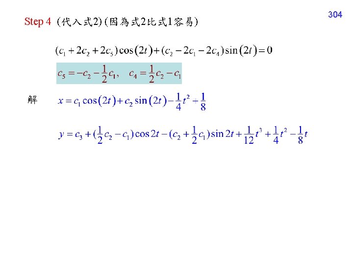
302 Example 2 (text page 171) (式 2) Step 1 Step 2 -1 (式 2) D − (式 1) Step 3 -1 complementary function: particular solution:
Step 2 -2 (式 1) (D+1) − (式 2) (D− 4) Step 3 -2 complementary function: particular solution 注意,不可設為 303
311 4 -9 Nonlinear Differential Equations Method 1: Reduction of Order Method 2: Taylor Series Method 3: Numerical Approach
4 -9 -1 Method 1: Reduction of Order 精神:變成 1 st order DE 再用 1 st order DE 的方法求解 (這方法的名字和 Section 4 -2 一樣,但是不限於 linear, 而且不必知道其中一個解) 限制:The DE should have the form of Case 1, page 313 Case 2, page 315 or (Without the term y) (Without the term x) 312
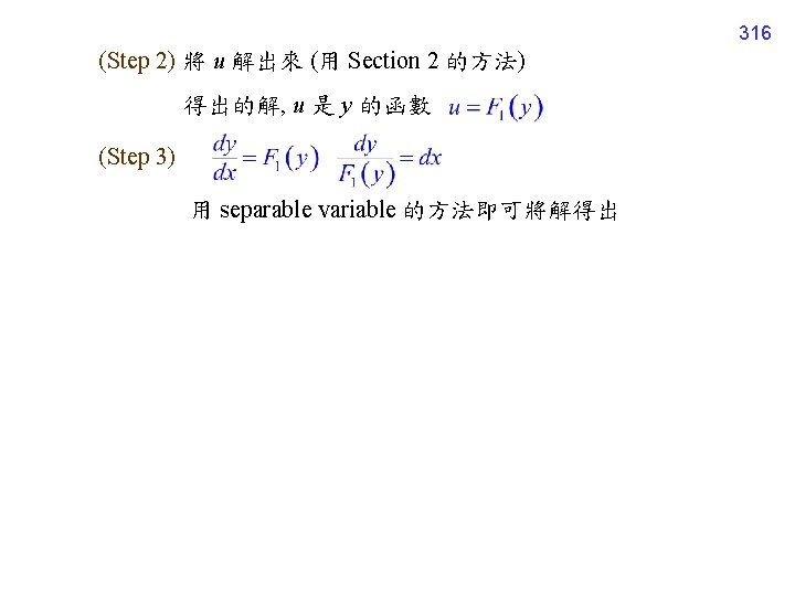
313 Case 1: The 2 nd order DE has the form of 解法: (Step 1) Set 此時DE 變成 (Without the term y) (對 u 而言,是 1 st order DE) (Step 2) 將 u 解出來 (用 Section 2 的方法) (Step 3) 對 u 作積分,即解出 y
314 Example 1 (text page 174) (Step 1) 問題: u 要用什麼方法解? (Step 2) (Step 3)
315 Case 2: The 2 nd order DE has the form of (Without the term x) 解法:(Step 1) Set (Chain rule) 此時DE 變成 (對 u 而言,是 1 st order DE, independent variable 為 y)
317 Example 2 (text page 175) (Step 1) Set (Step 2) (Step 3)
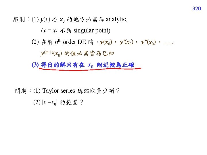
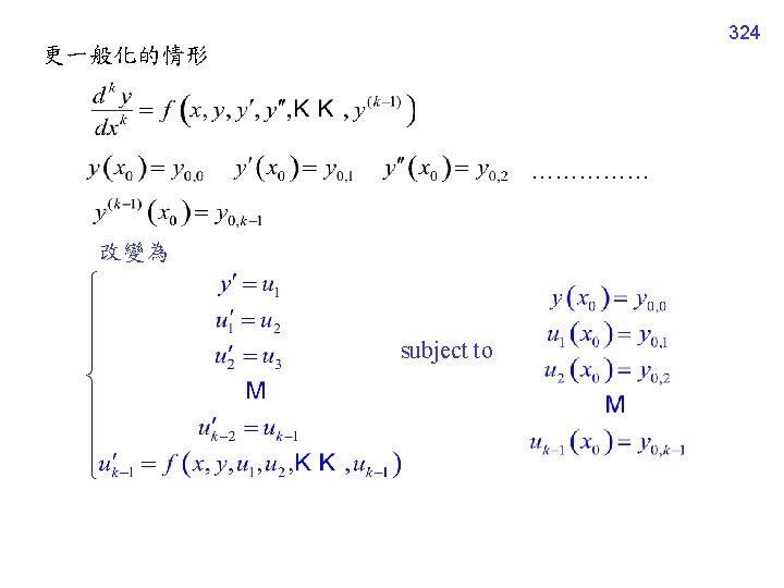
4 -9 -2 Method 2: Taylor Series 更一般化的型態 Step 1 算出 Step 2 代回 Taylor series 318
Example 3 (text page 176) : 代回 Taylor series 319
321 Figure 4. 9. 1
4 -9 -3 Method 3: Numerical Method 解法 subject to 使用Section 2 -6 的 Euler’s Method 322
323 Recursive 的解法 Initial: n=n+1 n=0
Recursive 的解法 n=n+1 325
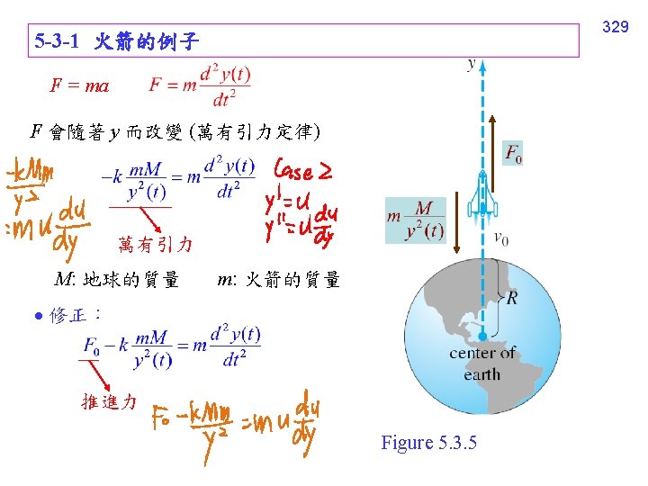
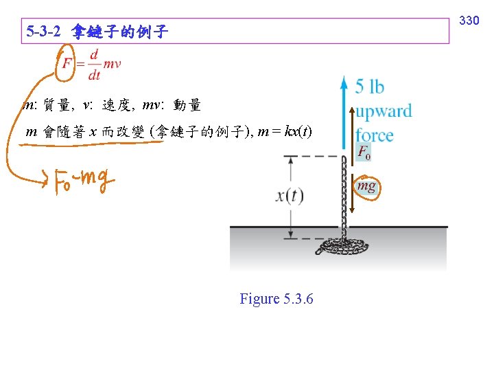
328 5 -3 Nonlinear Models 非線性彈簧的例子 (text pages 207, 208) 鍾擺的例子 (text pages 209, 210) 電話線的例子 (text pages 210, 211) 火箭的例子 (text pages 211) 拿鏈子的例子 (text pages 211, 212, 213)
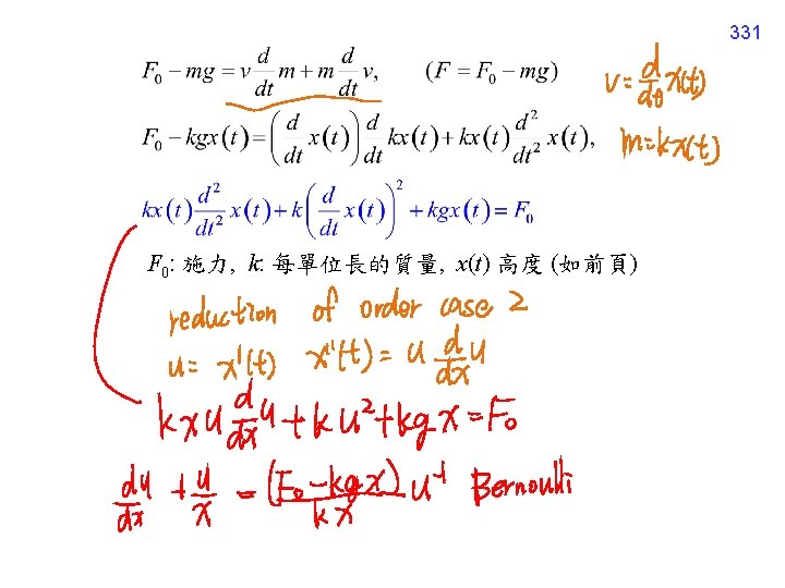
332 Example 4 (text page 212)
333 (1) Cauchy-Euler equation 缺乏應用 (2) 許多情形還是只能用 Numerical Method 來解
Reviews for Higher Order DE: (A) Linear DE Complementary Function 3 大解法 (1) Reduction of Order (Section 4 -2) 適用情形: (2) Auxiliary Function (Section 4 -3) 適用情形: 4 Cases (See pages 179, 180) 335
(3) Cauchy-Euler Equation (Section 4 -7) 適用情形: 336
(B) Linear DE Particular solution 3 大解法 (1) Guess (Section 4 -4) (熟悉講義 page 191 的表) 要訣: yp should be a linear combination of g(x), g'''(x), g(4)(x), g(5)(x), ……………. 適用情形: 遇到重覆,乘 x 或 lnx (2) Annihilator (Section 4 -5) 若原本的 DE 為 L[y(x)] = g(x) Annihilator: L 1[ g(x)] = 0 Particular solution 為 L 1{L[y(x)]} = 0 的解 (扣去和 L[y(x)] = 0 的解重複的部分) 適用情形: Annihilator 算法三大規則: Pages 210 -212 337
(3) Variation of parameters (Section 4 -6) Wk : replace the kth column of W by 適用情形: 338
(4) For Cauchy-Euler Equation (Section 4 -7) 可採用二種方法 (1) 先用 解 complementary function 再用 Variation of parameters 解 particular solution (2) Use the method on pages 253, 254 Set x = et, t = ln x 339
(C) Combination of Linear DEs (Section 4 -8) 方法: Step 1: 將 變成 Dn Steps 2, 3: 用代數消去法,變成只含有一個 dependent variable 的 DE,再將這個 dependent variable 解出來 Step 4: 代回原式,求各 dependent variable 的常數 ck 之間的 關係 適用情形: 340
(D) Nonlinear DE 的3大解法 (Section 4 -9) (1) Reduction of Order (1 -1) Set (1 -2) Set 341
342 (2) Taylor Series 適用情形: (3) Numerical Method 適用情形:
343 Exercises for practicing Section 4 -8 5, 10, 14, 17, 18, 20, 22, 23 Section 4 -9 1, 5, 6, 8, 11, 12, 15, 18, 19 Review 4 33, 34, 38, 40 Section 5 -1 11, 25, 40, 45 Section 5 -2 5, 22 Section 5 -3 14, 16 Review 5 21, 22