2 Digital Filter Design A noise operation filter

![(假設一) 41 Specially, when h[n] is even symmetric h[n] = h[N− 1 −n] and (假設一) 41 Specially, when h[n] is even symmetric h[n] = h[N− 1 −n] and](https://slidetodoc.com/presentation_image_h/cf10d100c3408e840db1e7337c855a16/image-5.jpg)
![42 Impulse Response of the FIR Filter: h[n] (h[n] 0 for 0 n N 42 Impulse Response of the FIR Filter: h[n] (h[n] 0 for 0 n N](https://slidetodoc.com/presentation_image_h/cf10d100c3408e840db1e7337c855a16/image-6.jpg)
![47 Minimize MSE Make for all n’s , . Finally, set h[k] = s[0], 47 Minimize MSE Make for all n’s , . Finally, set h[k] = s[0],](https://slidetodoc.com/presentation_image_h/cf10d100c3408e840db1e7337c855a16/image-11.jpg)
![(Step 2): From page 42, [R(Fm) Hd(Fm)]W(Fm) = 0, 1, 2, …. . , (Step 2): From page 42, [R(Fm) Hd(Fm)]W(Fm) = 0, 1, 2, …. . ,](https://slidetodoc.com/presentation_image_h/cf10d100c3408e840db1e7337c855a16/image-18.jpg)
![s [0] s [1] s [2] s [3] R(F) = 0. 5120 – 0. s [0] s [1] s [2] s [3] R(F) = 0. 5120 – 0.](https://slidetodoc.com/presentation_image_h/cf10d100c3408e840db1e7337c855a16/image-26.jpg)
![65 (Step 6) From s[0] = 0. 4990, s[1] = – 0. 6267, s[2] 65 (Step 6) From s[0] = 0. 4990, s[1] = – 0. 6267, s[2]](https://slidetodoc.com/presentation_image_h/cf10d100c3408e840db1e7337c855a16/image-29.jpg)
![67 (Step 2) s[0] = 0. 4638, s[1] = 0. 6327, s[2] = 0. 67 (Step 2) s[0] = 0. 4638, s[1] = 0. 6327, s[2] = 0.](https://slidetodoc.com/presentation_image_h/cf10d100c3408e840db1e7337c855a16/image-31.jpg)
![69 After 7 times of iteration s[0] = 0. 4243, s[1] = 0. 7559, 69 After 7 times of iteration s[0] = 0. 4243, s[1] = 0. 7559,](https://slidetodoc.com/presentation_image_h/cf10d100c3408e840db1e7337c855a16/image-33.jpg)
![附錄二:Spectrum Analysis for Sampled Signals (學信號處理的人一定要會的基本常識) 已知 x[n] 是由一個 continuous signal y(t) 取樣而得 x[n] 附錄二:Spectrum Analysis for Sampled Signals (學信號處理的人一定要會的基本常識) 已知 x[n] 是由一個 continuous signal y(t) 取樣而得 x[n]](https://slidetodoc.com/presentation_image_h/cf10d100c3408e840db1e7337c855a16/image-34.jpg)
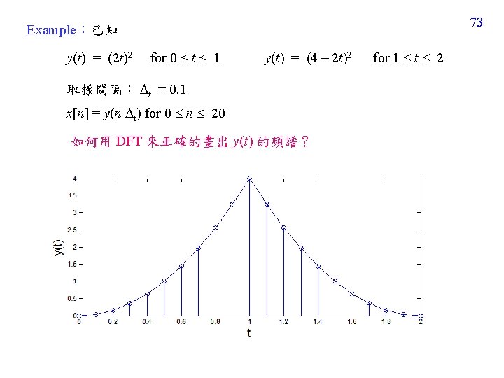
![74 x[n] = y(n t) for 0 n 20 (Step 1) Perform the DFT 74 x[n] = y(n t) for 0 n 20 (Step 1) Perform the DFT](https://slidetodoc.com/presentation_image_h/cf10d100c3408e840db1e7337c855a16/image-38.jpg)
- Slides: 39

2. Digital Filter Design (A) 任何可以用來去除 noise 作用的 operation,皆被稱為 filter 甚至有部分的 operation,雖然主要功用不是用來去除 noise,但是 可以用 FT + multiplication + IFT 來表示,也被稱作是 filter = convolution, LTI system Reference [1] A. V. Oppenheim and R. W. Schafer, Discrete-Time Signal Processing, London: Prentice-Hall, 3 rd ed. , 2010. [2] D. G. Manolakis and V. K. Ingle, Applied Digital Signal Processing, Cambridge University Press, Cambridge, UK. 2011. [3] B. A. Shenoi, Introduction to Digital Signal Processing and Filter Design, Wiley-Interscience, N. J. , 2006. [4] A. A. Khan, Digital Signal Processing Fundamentals, Da Vinci Engineering Press, Massachusetts, 2005. [5] S. Winder, Analog and Digital Filter Design, 2 nd Ed. , Amsterdam, 2002. 37

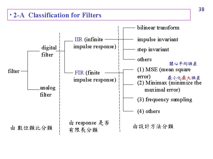
38 2 -A Classification for Filters bilinear transform digital filter IIR (infinite impulse response) impulse invariant step invariant others FIR (finite impulse response) analog filter 關心平均誤差 (1) MSE (mean square error) 最小化最大誤差 (2) Minimax (minimize the maximal error) (3) frequency sampling (4) others 由 數位類比分類 由 response 是否 有限長分類 由設計方法分類

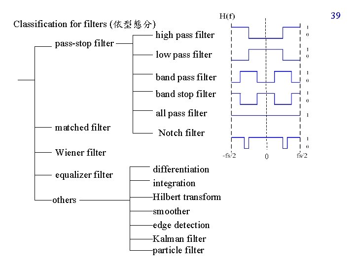
39 Classification for filters (依型態分) pass-stop filter high pass filter low pass filter band stop filter all pass filter matched filter Notch filter Wiener filter equalizer filter others 0 differentiation integration Hilbert transform smoother edge detection Kalman filter particle filter

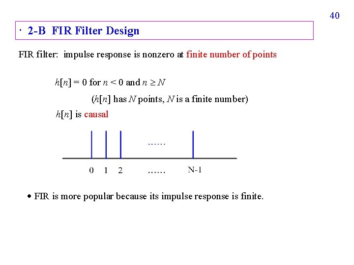
40 2 -B FIR Filter Design FIR filter: impulse response is nonzero at finite number of points h[n] = 0 for n < 0 and n N (h[n] has N points, N is a finite number) h[n] is causal FIR is more popular because its impulse response is finite.
![假設一 41 Specially when hn is even symmetric hn hN 1 n and (假設一) 41 Specially, when h[n] is even symmetric h[n] = h[N− 1 −n] and](https://slidetodoc.com/presentation_image_h/cf10d100c3408e840db1e7337c855a16/image-5.jpg)
(假設一) 41 Specially, when h[n] is even symmetric h[n] = h[N− 1 −n] and N is an odd number (假設二) h[-1] h[0] h[1] h[k-2] h[k-1] h[k+1] h[k+2] r[-k-1] r[-k+1] r[-2] r[-1] r[0] r[1] s[0] s[1]/2 (a) r[n] = h[n + k], (b) s[0] = r[0], r[2] s[2]/2 where k = (N 1)/2. s[n] = 2 r[n] for 0 < n k. h[N-2] h[N-1] h[N+1] r[k-1] r[k+1] r[k+2] s[k-1]/2 s[k]/2
![42 Impulse Response of the FIR Filter hn hn 0 for 0 n N 42 Impulse Response of the FIR Filter: h[n] (h[n] 0 for 0 n N](https://slidetodoc.com/presentation_image_h/cf10d100c3408e840db1e7337c855a16/image-6.jpg)
42 Impulse Response of the FIR Filter: h[n] (h[n] 0 for 0 n N 1) r[n] = h[n + k], k = (N 1)/2 (r[n] 0 for -k n k, see page 41) Suppose that the filter is even, r[n] = r[ n]. Set s[0] = r[0], s[n] = 2 r[n] for n 0. Then, the discrete-time Fourier transform of the filter is (F = f t is the normalized frequency) See page 22

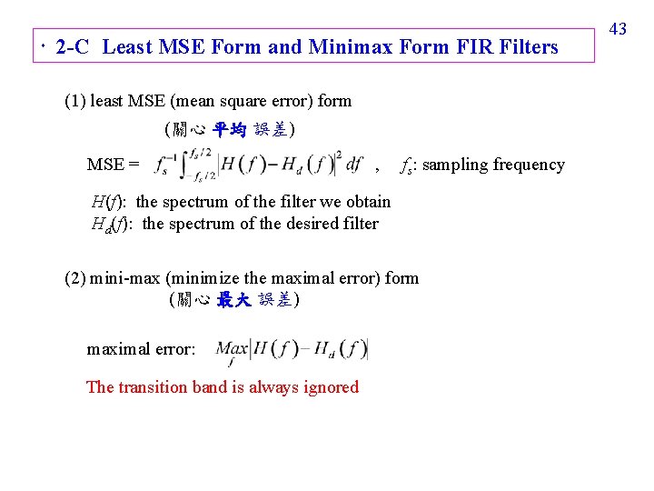
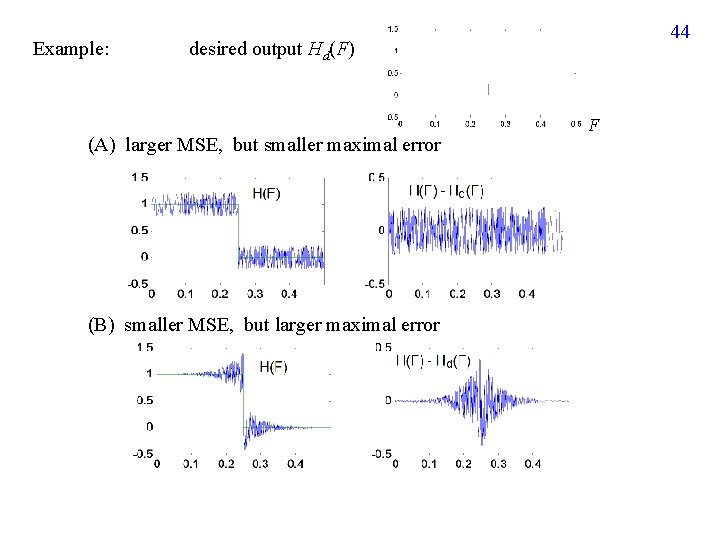
2 -C Least MSE Form and Minimax Form FIR Filters (1) least MSE (mean square error) form (關心 平均 誤差) MSE = , fs: sampling frequency H(f): the spectrum of the filter we obtain Hd(f): the spectrum of the desired filter (2) mini-max (minimize the maximal error) form (關心 最大 誤差) maximal error: The transition band is always ignored 43

Example: 44 desired output Hd(F) (A) larger MSE, but smaller maximal error (B) smaller MSE, but larger maximal error F

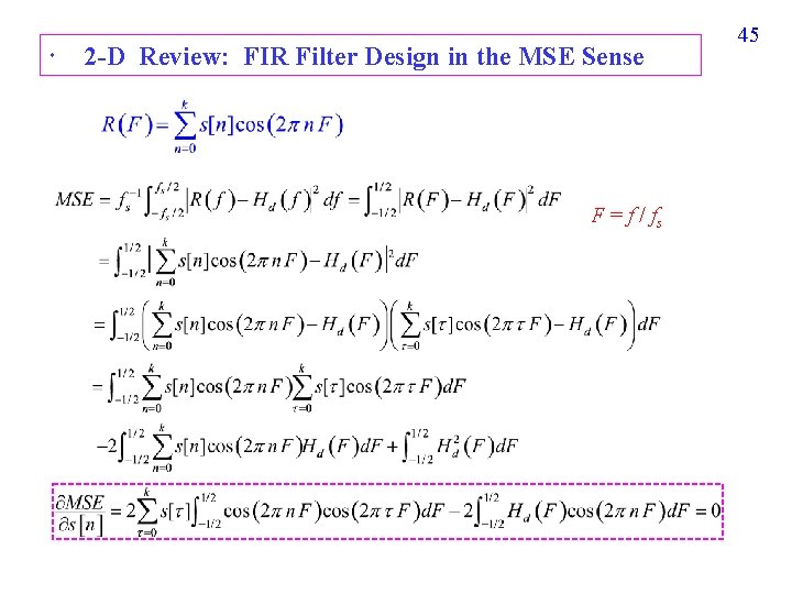
2 -D Review: FIR Filter Design in the MSE Sense F = f / fs 45

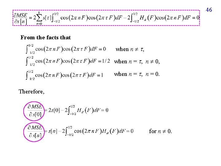
46 From the facts that when n , when n = , n 0, when n = , n = 0. Therefore, for n 0.
![47 Minimize MSE Make for all ns Finally set hk s0 47 Minimize MSE Make for all n’s , . Finally, set h[k] = s[0],](https://slidetodoc.com/presentation_image_h/cf10d100c3408e840db1e7337c855a16/image-11.jpg)
47 Minimize MSE Make for all n’s , . Finally, set h[k] = s[0], h[k+n] = s[n]/2, h[k n] = s[n]/2 for n = 1, 2, 3, …. , k, h[n] = 0 for n < 0 and n N. Then, h[n] is the impulse response of the designed filter.

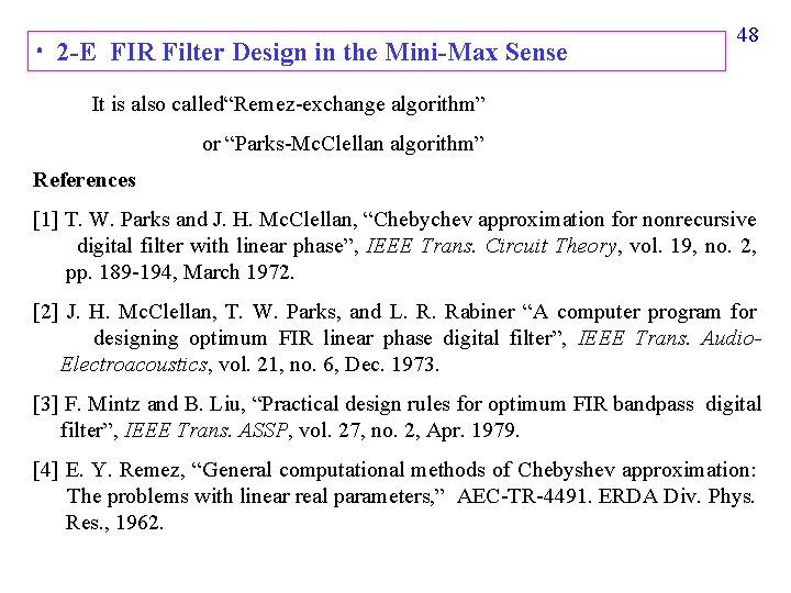
2 -E FIR Filter Design in the Mini-Max Sense 48 It is also called“Remez-exchange algorithm” or “Parks-Mc. Clellan algorithm” References [1] T. W. Parks and J. H. Mc. Clellan, “Chebychev approximation for nonrecursive digital filter with linear phase”, IEEE Trans. Circuit Theory, vol. 19, no. 2, pp. 189 -194, March 1972. [2] J. H. Mc. Clellan, T. W. Parks, and L. R. Rabiner “A computer program for designing optimum FIR linear phase digital filter”, IEEE Trans. Audio. Electroacoustics, vol. 21, no. 6, Dec. 1973. [3] F. Mintz and B. Liu, “Practical design rules for optimum FIR bandpass digital filter”, IEEE Trans. ASSP, vol. 27, no. 2, Apr. 1979. [4] E. Y. Remez, “General computational methods of Chebyshev approximation: The problems with linear real parameters, ” AEC-TR-4491. ERDA Div. Phys. Res. , 1962.

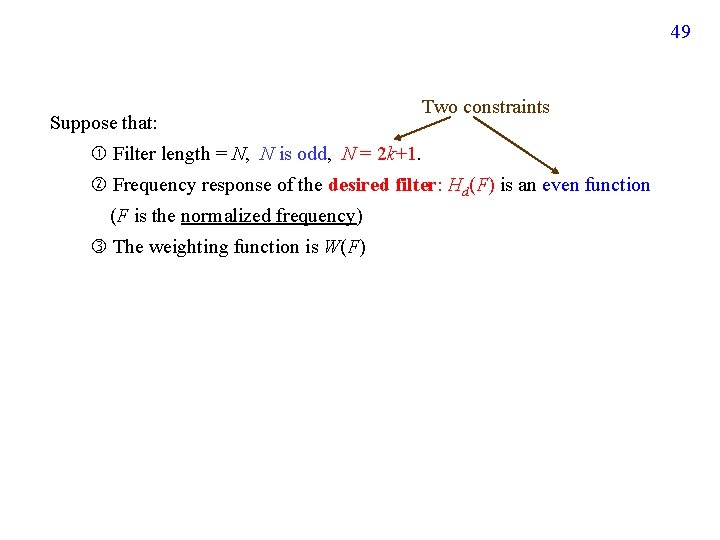
49 Suppose that: Two constraints Filter length = N, N is odd, N = 2 k+1. Frequency response of the desired filter: Hd(F) is an even function (F is the normalized frequency) The weighting function is W(F)

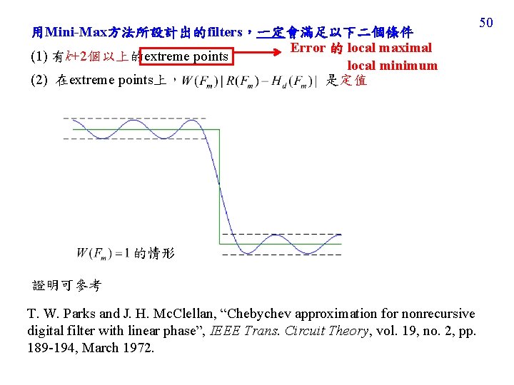
用Mini-Max方法所設計出的filters,一定會滿足以下二個條件 Error 的 local maximal (1) 有k+2個以上的extreme points local minimum (2) 在extreme points上, 是定值 的情形 證明可參考 T. W. Parks and J. H. Mc. Clellan, “Chebychev approximation for nonrecursive digital filter with linear phase”, IEEE Trans. Circuit Theory, vol. 19, no. 2, pp. 189 -194, March 1972. 50

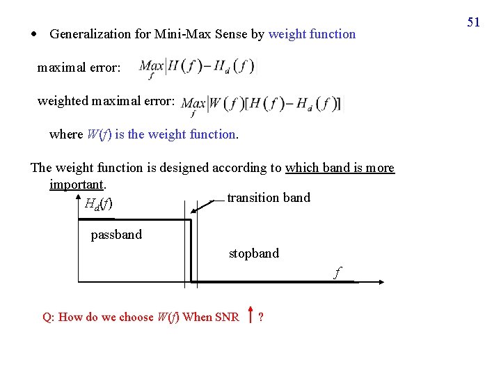
Generalization for Mini-Max Sense by weight function maximal error: weighted maximal error: where W(f) is the weight function. The weight function is designed according to which band is more important. transition band Hd(f) passband stopband f Q: How do we choose W(f) When SNR ? 51

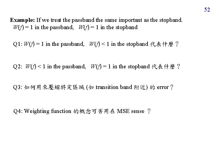
52 Example: If we treat the passband the same important as the stopband. W(f) = 1 in the passband, W(f) = 1 in the stopband Q 1: W(f) = 1 in the passband, W(f) < 1 in the stopband 代表什麼? Q 2: W(f) < 1 in the passband, W(f) = 1 in the stopband 代表什麼? Q 3: 如何用來壓縮特定區域 (如 transition band 附近) 的 error? Q 4: Weighting function 的概念可否用在 MSE sense ?

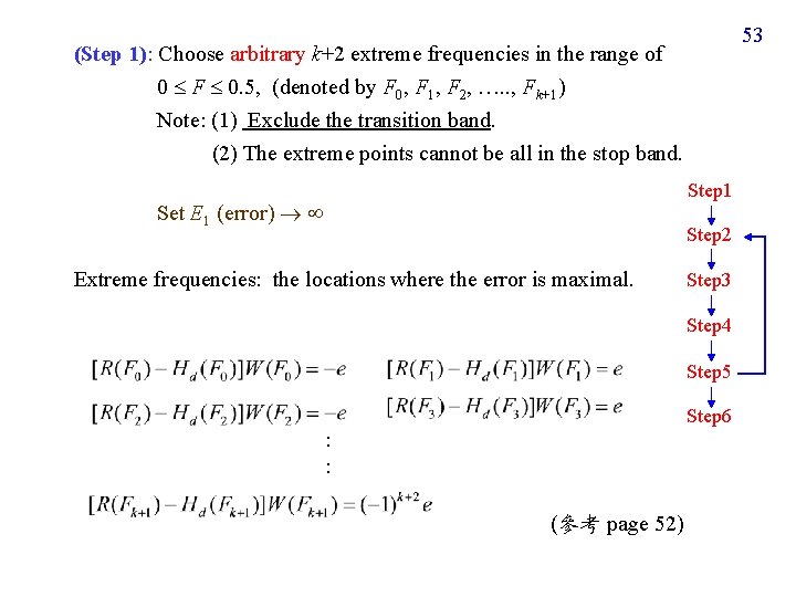
53 (Step 1): Choose arbitrary k+2 extreme frequencies in the range of 0 F 0. 5, (denoted by F 0, F 1, F 2, …. . , Fk+1) Note: (1) Exclude the transition band. (2) The extreme points cannot be all in the stop band. Step 1 Set E 1 (error) Step 2 Extreme frequencies: the locations where the error is maximal. Step 3 Step 4 Step 5 Step 6 : : (參考 page 52)
![Step 2 From page 42 RFm HdFmWFm 0 1 2 (Step 2): From page 42, [R(Fm) Hd(Fm)]W(Fm) = 0, 1, 2, …. . ,](https://slidetodoc.com/presentation_image_h/cf10d100c3408e840db1e7337c855a16/image-18.jpg)
(Step 2): From page 42, [R(Fm) Hd(Fm)]W(Fm) = 0, 1, 2, …. . , k+1) can be written as ( 1)m+1 e (where m = 54 where m = 0, 1, 2, …. . , k+1. Expressed by the matrix form: Solve s[0], s[1], s[2], …. . , s[k] from the above matrix (performing the matrix inversion). Square matrix

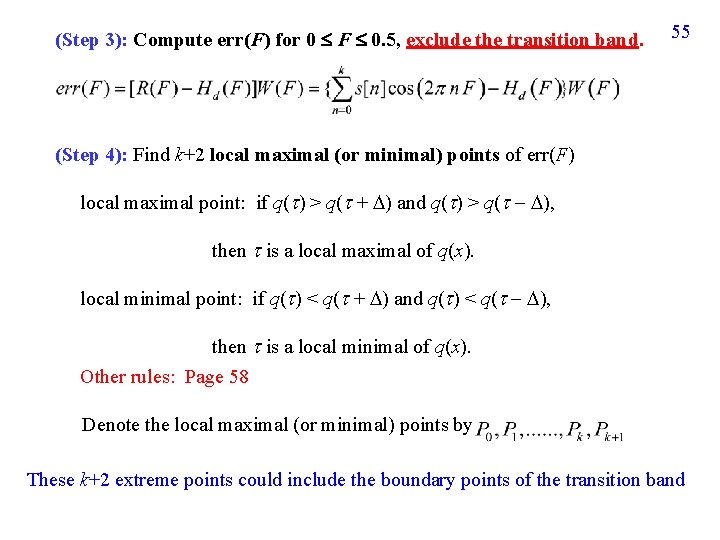
(Step 3): Compute err(F) for 0 F 0. 5, exclude the transition band. 55 (Step 4): Find k+2 local maximal (or minimal) points of err(F) local maximal point: if q( ) > q( + ) and q( ) > q( ), then is a local maximal of q(x). local minimal point: if q( ) < q( + ) and q( ) < q( ), then is a local minimal of q(x). Other rules: Page 58 Denote the local maximal (or minimal) points by These k+2 extreme points could include the boundary points of the transition band

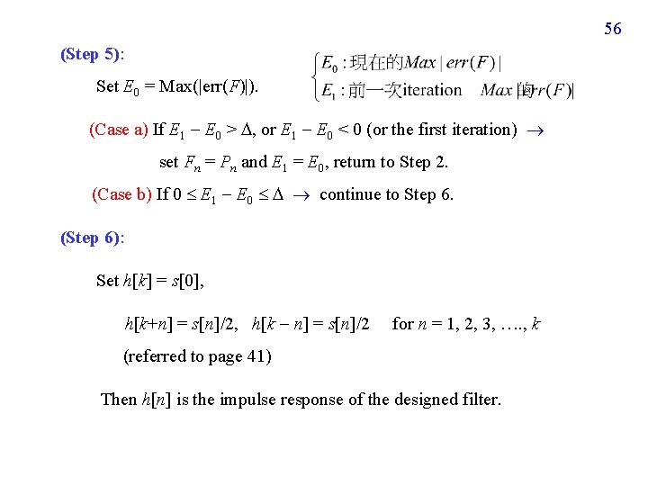
56 (Step 5): Set E 0 = Max(|err(F)|). (Case a) If E 1 E 0 > , or E 1 E 0 < 0 (or the first iteration) set Fn = Pn and E 1 = E 0, return to Step 2. (Case b) If 0 E 1 E 0 continue to Step 6. (Step 6): Set h[k] = s[0], h[k+n] = s[n]/2, h[k n] = s[n]/2 for n = 1, 2, 3, …. , k (referred to page 41) Then h[n] is the impulse response of the designed filter.

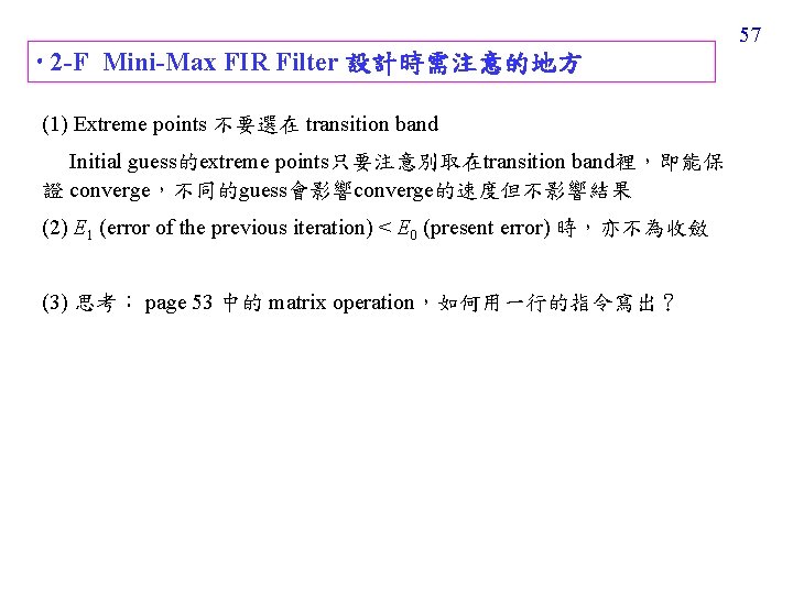
57 2 -F Mini-Max FIR Filter 設計時需注意的地方 (1) Extreme points 不要選在 transition band Initial guess的extreme points只要注意別取在transition band裡,即能保 證 converge,不同的guess會影響converge的速度但不影響結果 (2) E 1 (error of the previous iteration) < E 0 (present error) 時,亦不為收斂 (3) 思考: page 53 中的 matrix operation,如何用一行的指令寫出?

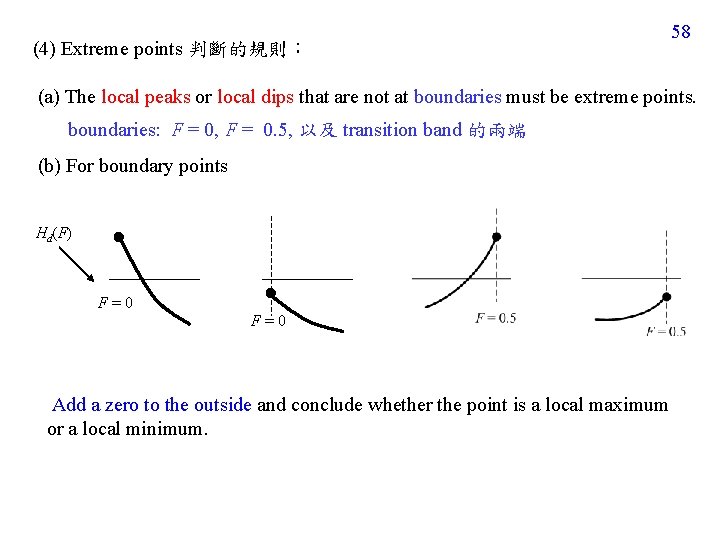
(4) Extreme points 判斷的規則: 58 (a) The local peaks or local dips that are not at boundaries must be extreme points. boundaries: F = 0, F = 0. 5, 以及 transition band 的兩端 (b) For boundary points Hd(F) F=0 Add a zero to the outside and conclude whether the point is a local maximum or a local minimum.

59 (5) 有時,會找到多於 k+2 個 extreme points, 該如何選 (a) 優先選擇不在 boundaries 的 extreme points (b) 其次選擇 boundary extreme points 當中 |err(F)| 較大的, 直到湊足 k+2 個 extreme points 為止 (c) 在 boundary extreme points 的 |err(F)| 一樣大的情形, 優先選擇 transition bands 兩旁的點

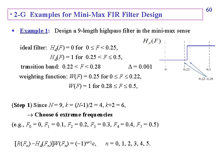
2 -G Examples for Mini-Max FIR Filter Design Example 1: Design a 9 -length highpass filter in the mini-max sense ideal filter: Hd(F) = 0 for 0 F < 0. 25, Hd(F) = 1 for 0. 25 < F 0. 5, = 0. 001 transition band: 0. 22 < F < 0. 28 weighting function: W(F) = 0. 25 for 0 F 0. 22, W(F) = 1 for 0. 28 F 0. 5, (Step 1) Since N = 9, k = (N-1)/2 = 4, k+2 = 6, Choose 6 extreme frequencies (e. g. , F 0 = 0, F 1 = 0. 1, F 2 = 0. 2, F 3 = 0. 3, F 4 = 0. 4, F 5 = 0. 5) [R(Fn) Hd(Fn)]W(Fn) = ( 1)n+1 e, n = 0, 1, 2, 3, 4, 5. 60

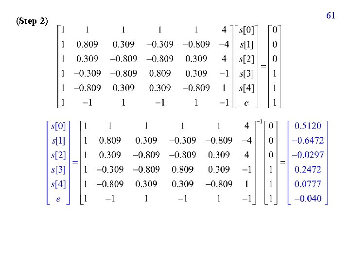
(Step 2) 61
![s 0 s 1 s 2 s 3 RF 0 5120 0 s [0] s [1] s [2] s [3] R(F) = 0. 5120 – 0.](https://slidetodoc.com/presentation_image_h/cf10d100c3408e840db1e7337c855a16/image-26.jpg)
s [0] s [1] s [2] s [3] R(F) = 0. 5120 – 0. 6472 cos(2 F) – 0. 0297 cos(4 F) + 0. 2472 cos(6 F) + 0. 0777 cos(8 F) s [4] (Step 3) err(F) = [R(F) – Hd(F)]W(F) err(F) W[F] = 0 for 0. 22 < F < 0. 28 62

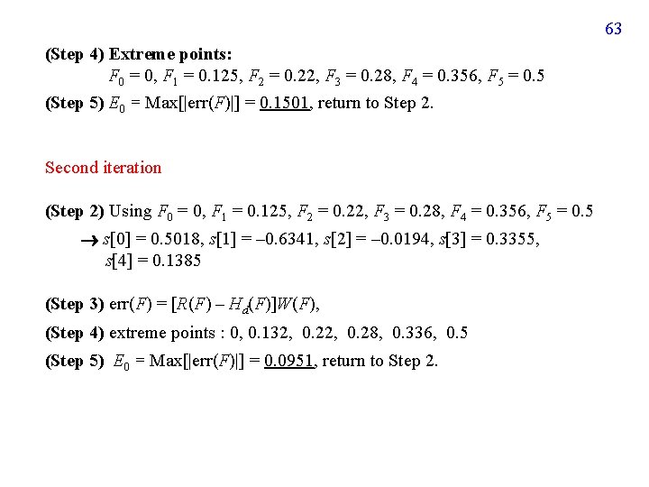
63 (Step 4) Extreme points: F 0 = 0, F 1 = 0. 125, F 2 = 0. 22, F 3 = 0. 28, F 4 = 0. 356, F 5 = 0. 5 (Step 5) E 0 = Max[|err(F)|] = 0. 1501, return to Step 2. Second iteration (Step 2) Using F 0 = 0, F 1 = 0. 125, F 2 = 0. 22, F 3 = 0. 28, F 4 = 0. 356, F 5 = 0. 5 s[0] = 0. 5018, s[1] = – 0. 6341, s[2] = – 0. 0194, s[3] = 0. 3355, s[4] = 0. 1385 (Step 3) err(F) = [R(F) – Hd(F)]W(F), (Step 4) extreme points : 0, 0. 132, 0. 28, 0. 336, 0. 5 (Step 5) E 0 = Max[|err(F)|] = 0. 0951, return to Step 2.

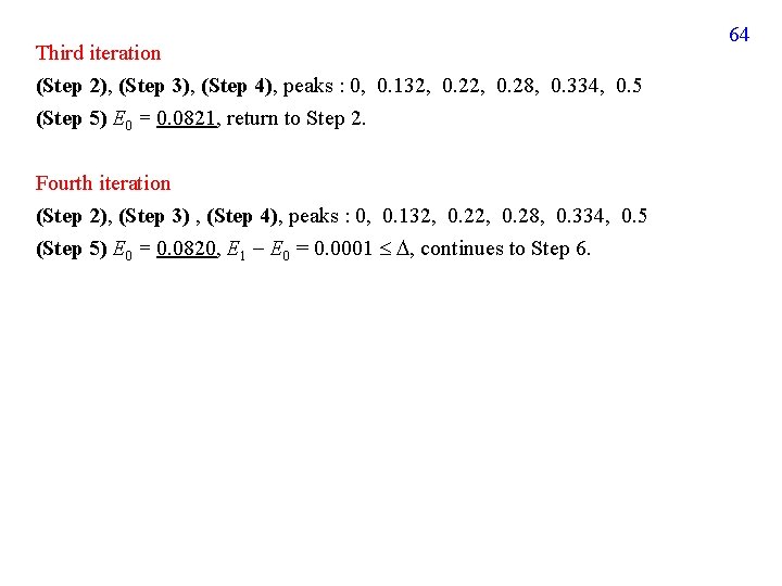
Third iteration (Step 2), (Step 3), (Step 4), peaks : 0, 0. 132, 0. 28, 0. 334, 0. 5 (Step 5) E 0 = 0. 0821, return to Step 2. Fourth iteration (Step 2), (Step 3) , (Step 4), peaks : 0, 0. 132, 0. 28, 0. 334, 0. 5 (Step 5) E 0 = 0. 0820, E 1 E 0 = 0. 0001 , continues to Step 6. 64
![65 Step 6 From s0 0 4990 s1 0 6267 s2 65 (Step 6) From s[0] = 0. 4990, s[1] = – 0. 6267, s[2]](https://slidetodoc.com/presentation_image_h/cf10d100c3408e840db1e7337c855a16/image-29.jpg)
65 (Step 6) From s[0] = 0. 4990, s[1] = – 0. 6267, s[2] = – 0. 0203, s[3] = 0. 3316, s[4] = 0. 1442 h[4] = s[0] = 0. 4990, h[2] = h[6] = s[2]/2 = – 0. 0101, h[0] = h[8] = s[4]/2 = 0. 0721. h[3] = h[5] = s[1]/2 = – 0. 3134, h[1] = h[7] = s[3]/2 = 0. 1658,

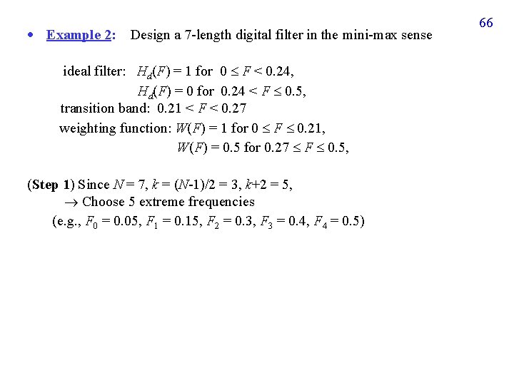
Example 2: Design a 7 -length digital filter in the mini-max sense ideal filter: Hd(F) = 1 for 0 F < 0. 24, Hd(F) = 0 for 0. 24 < F 0. 5, transition band: 0. 21 < F < 0. 27 weighting function: W(F) = 1 for 0 F 0. 21, W(F) = 0. 5 for 0. 27 F 0. 5, (Step 1) Since N = 7, k = (N-1)/2 = 3, k+2 = 5, Choose 5 extreme frequencies (e. g. , F 0 = 0. 05, F 1 = 0. 15, F 2 = 0. 3, F 3 = 0. 4, F 4 = 0. 5) 66
![67 Step 2 s0 0 4638 s1 0 6327 s2 0 67 (Step 2) s[0] = 0. 4638, s[1] = 0. 6327, s[2] = 0.](https://slidetodoc.com/presentation_image_h/cf10d100c3408e840db1e7337c855a16/image-31.jpg)
67 (Step 2) s[0] = 0. 4638, s[1] = 0. 6327, s[2] = 0. 0809, s[3] = -0. 1608, e = -0. 0364 R(F)

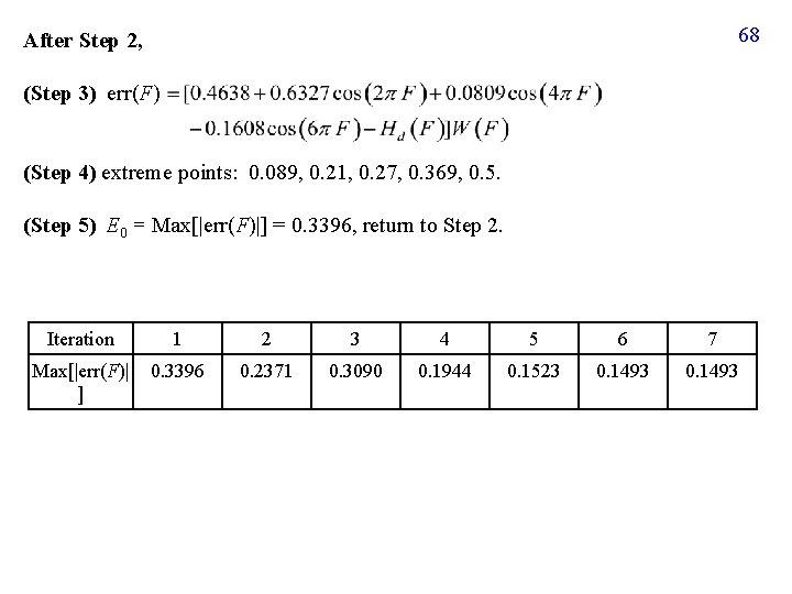
68 After Step 2, (Step 3) err(F) (Step 4) extreme points: 0. 089, 0. 21, 0. 27, 0. 369, 0. 5. (Step 5) E 0 = Max[|err(F)|] = 0. 3396, return to Step 2. Iteration 1 2 3 4 5 6 7 Max[|err(F)| ] 0. 3396 0. 2371 0. 3090 0. 1944 0. 1523 0. 1493
![69 After 7 times of iteration s0 0 4243 s1 0 7559 69 After 7 times of iteration s[0] = 0. 4243, s[1] = 0. 7559,](https://slidetodoc.com/presentation_image_h/cf10d100c3408e840db1e7337c855a16/image-33.jpg)
69 After 7 times of iteration s[0] = 0. 4243, s[1] = 0. 7559, s[2] = -0. 0676, s[3] = -0. 2619, e = 0. 1493 (Step 6): h[3] = 0. 4243, h[2] = h[4] = s[1]/2 = 0. 3780, h[1] = h[5] = s[2]/2 = -0. 0338, h[0] = h[6] = s[3]/2 = -0. 1309, h[n] = 0 for n < 0 and n > 6
![附錄二Spectrum Analysis for Sampled Signals 學信號處理的人一定要會的基本常識 已知 xn 是由一個 continuous signal yt 取樣而得 xn 附錄二:Spectrum Analysis for Sampled Signals (學信號處理的人一定要會的基本常識) 已知 x[n] 是由一個 continuous signal y(t) 取樣而得 x[n]](https://slidetodoc.com/presentation_image_h/cf10d100c3408e840db1e7337c855a16/image-34.jpg)
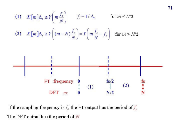
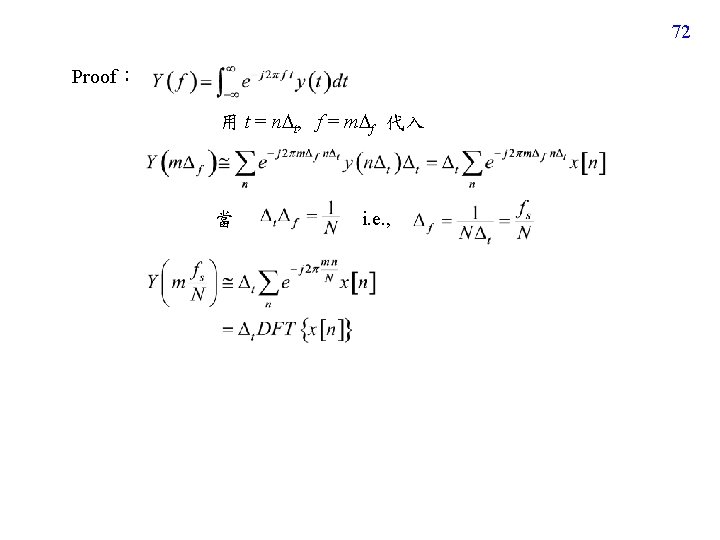
附錄二:Spectrum Analysis for Sampled Signals (學信號處理的人一定要會的基本常識) 已知 x[n] 是由一個 continuous signal y(t) 取樣而得 x[n] = y(n t) DFT: Q: x[n] 的 DFT 和 y(t) 的 Fourier transform 之間有什麼關係? Basic rule:把間隔由 1 換成 fs /N where fs = 1/ t (Very important) 70

71 fs = 1/ t (1) for m N/2 (2) for m > N/2 FT frequency 0 DFT m: 0 fs/2 (1) (2) N/2 If the sampling frequency is fs, the FT output has the period of fs The DFT output has the period of N fs N


![74 xn yn t for 0 n 20 Step 1 Perform the DFT 74 x[n] = y(n t) for 0 n 20 (Step 1) Perform the DFT](https://slidetodoc.com/presentation_image_h/cf10d100c3408e840db1e7337c855a16/image-38.jpg)
74 x[n] = y(n t) for 0 n 20 (Step 1) Perform the DFT for x[n] N = 21

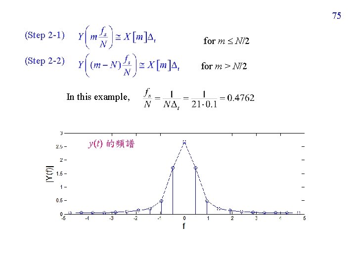
75 (Step 2 -1) for m N/2 (Step 2 -2) for m > N/2 In this example, y(t) 的頻譜