Correlation Regression The Data http core ecu edupsycwuenschkSPSS

Correlation & Regression

The Data • http: //core. ecu. edu/psyc/wuenschk/SPSS/ SPSS-Data. htm • Cyberloafing • See Correlation and Regression Analysis: SPSS • Master’s Thesis, Mike Sage, 2015 • Cyberloafing = Age, Conscientiousness

Analyze, Correlate, Bivariate

Pearson Correlations Cyberloafing Pearson Correlation Cyberloafing Sig. (2 -tailed) 1 Age -. 563** . 001 . 000 51 51 51 -. 462** 1 . 143 . 001 Sig. (2 -tailed) N Pearson Correlation Conscientiousness -. 462** N Pearson Correlation Age . 317 51 51 51 -. 563** . 143 1 Sig. (2 -tailed) N **. Correlation is significant at the 0. 01 level (2 -tailed). . 000 51 . 317 51 51

Spearman Correlations Cyberloafing Correlation Coefficient Spearman's rho Age Sig. (2 -tailed) N Correlation Coefficient Conscientiousness 1. 000 Sig. (2 -tailed) N **. Correlation is significant at the 0. 01 level (2 -tailed). Conscientiousness -. 431** -. 551** . 002 . 000 51 51 51 -. 431** 1. 000 . 110 Sig. (2 -tailed) N Age . . 002 . . 442 51 51 51 -. 551** . 110 1. 000 . 442 51 51

Analyze, Regression, Linear

Statistics

Plots

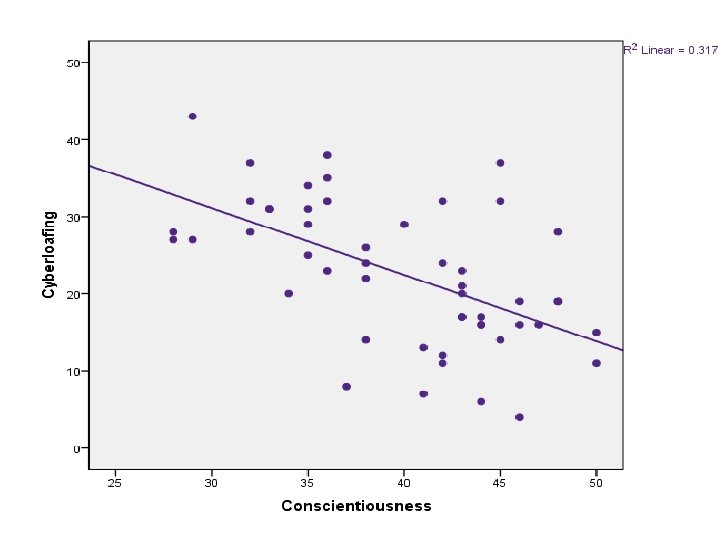
Model Summaryb Model R R Square Adjusted R Square 1. 563 a. 317 a. Predictors: (Constant), Conscientiousness Std. Error of the Estimate . 303 b. Dependent Variable: Cyberloafing r =. 1 is small, . 3 medium, . 5 large 7. 677

ANOVAa Sum of Squares Model Regression 1339. 801 1 df 1 Mean Square F Sig. 1339. 801 22. 736. 000 b Residual 2887. 532 49 58. 929 Total 4227. 333 50 a. Dependent Variable: Cyberloafing b. Predictors: (Constant), Conscientiousness

Coefficientsa Model Unstandardized Coefficients B 1 (Constant) Conscientiousness a. Dependent Variable: Cyberloafing 57. 039 -. 864 Std. Error Standardized Coefficients -. 563 7. 826 . 000 -4. 768 . 000 Cyberloafing = 57. 039 -. 864(Conscientiousness) + error t. Consc. =. 864/. 181 = 4. 77 = SQRT(22. 736) = SQRT(F) Sig. Beta 7. 288 . 181 t

Residuals Histogram

Graphs, Scatter, Simple, Define

Chart Editor, Elements, Fit Line at Total, Method = Linear, Close

Construct a Confidence Interval for the calculator at Vassar

Trivariate Analysis

Statistics

Plots

R 2 • Adding Age increased R 2 from. 317 to. 466. Model 1 R R Square . 682 a . 466 Adjusted R Square. 443

ANOVAa Model 1 Sum of Squares df Mean Square Regression 1968. 029 2 Residual 2259. 304 48 Total 4227. 333 50 F Sig. 984. 015 20. 906 . 000 b 47. 069

Coefficients Model Unstandardized Coefficients B (Constant) 1 Std. Error 64. 066 6. 792 Conscientiousness -. 779 . 164 Age -. 276 . 075

Unstandardized Coefficients • Cyberloaf = 64. 07 -. 78 Consc -. 28 Age • When Consc and Age = 0, Cyber = 64. 07 • Holding Age constant, each one point increase in Consc produces a. 78 point decrease in Cyberloafing. • Holding Consc constant, each one point increase in Age produces a. 28 point decrease in Cyberloafing.

How Large are these Effects? • Is a. 78 drop in Cyberloafing a big drop or a small drop? • When the units of measurement are arbitrary and not very familiar to others, best to standardize the coefficients to mean 0, standard deviation 1. • ZCyber = 0 + 1 Consc + 2 Age

More Coefficients Beta Constant Conscie Age t Sig. Correlations Zero-order Partial Part 9. 433 . 000 -. 507 -4. 759 . 000 -. 563 -. 566 -. 502 -. 389 -3. 653 . 001 -. 462 -. 466 -. 386

Beta Weights • ZCyber = 0 -. 51 Consc -. 39 Age • Holding Age constant, each one SD increase in Conscientiousness produces a . 51 SD decrease in Cyberloafing • Holding Conscientiousness constant, each one SD increase in Age produces a. 39 SD decrease in Cyberloafing.

Semi-Partial Correlations • The correlation between all of Cyberloafing and that part of Conscientiousness that is not related to Age = -. 50. • The correlation between all of Cyberloafing and that part of Age that is not related to Conscientiousness = -. 39.

Partial Correlations • The correlation between that part of Cyberloafing that is not related to Age and that part of Conscientiousness that is not related to Age = -. 57. • The correlation between that part of Cyberloafing that is not related to Conscientiousness and that part of Age that is not related to Conscientiousness = -. 47.

Multicollinearity • The R 2 between any one predictor and the remaining predictors is very high. • Makes the solution unstable. • Were you to repeatedly get samples from the same population, the regression coefficients would vary greatly among samples

Collinearity Diagnostics • Tolerance, which is simply 1 minus the R 2 between one predictor and the remaining predictors. Low (. 1) is troublesome. • VIF, the Variance Inflation Factor, is the reciprocal of tolerance. High (10) is troublesome.

Coefficientsa Model Collinearity Statistics Tolerance VIF Age . 980 1. 021 Conscientiousness . 980 1. 021 1

Residuals Statisticsa Predicted Value Minimum Maximum Mean Std. Deviation N 10. 22 35. 41 22. 67 6. 274 51 -17. 344 15. 153 . 000 6. 722 51 Std. Predicted Value -1. 983 2. 032 . 000 1. 000 51 Std. Residual -2. 528 2. 209 . 000 . 980 51 Residual No standardized residuals beyond 3 SD.

Residuals Histogram

Residuals Plot

Put a CI on R 2 • http: //core. ecu. edu/psyc/wuenschk/SPSS/ SPSS-Programs. htm • CI-R 2 -SPSS. zip -- Construct Confidence Interval for R 2 from regression analysis – Using SPSS to Obtain a Confidence Interval for R 2 From Regression -- instructions – Nonc. F. sav -- necessary data file – F 2 R 2. sps -- see Smithson's Workshop – Nonc. F 3. sps -- syntax file

Open Nonc. F. sav • Enter the observed value of F and degrees of freedom.

Open and Run the Syntax

Look Back at. sav File

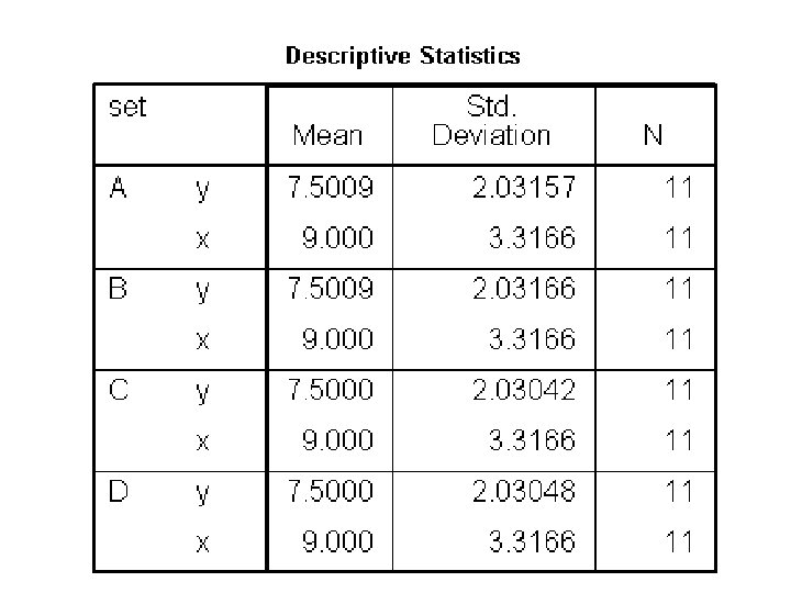
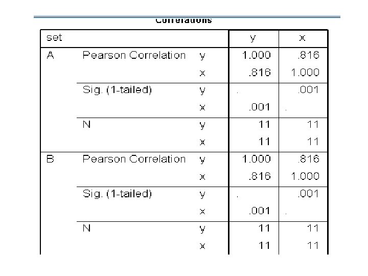
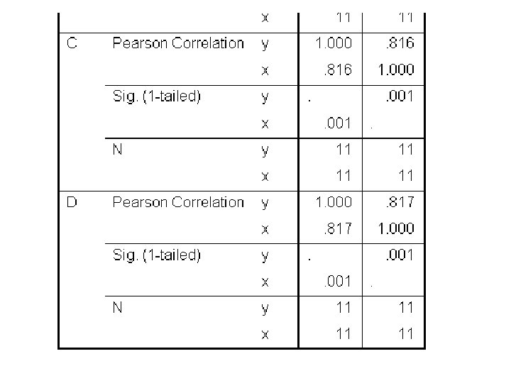
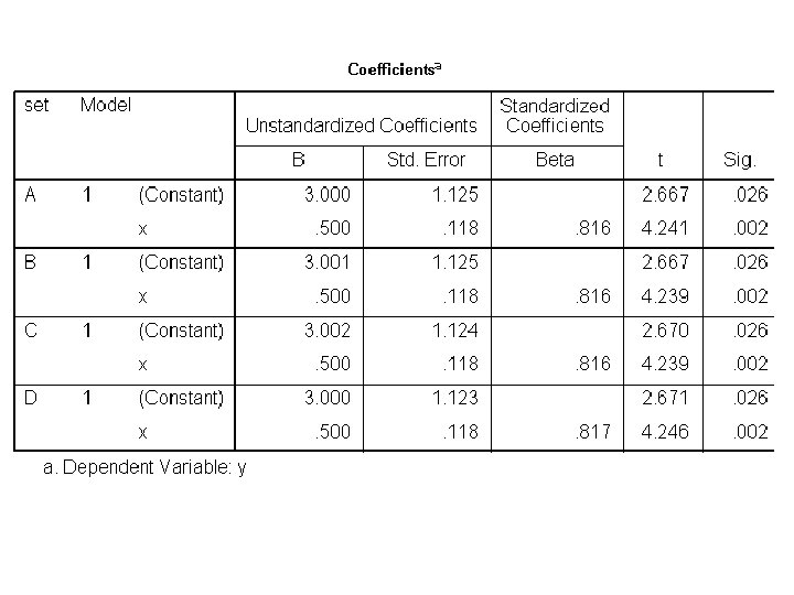
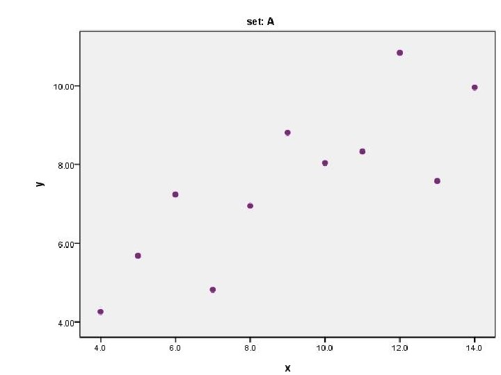
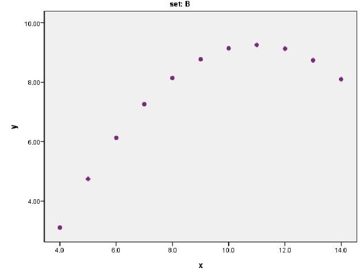
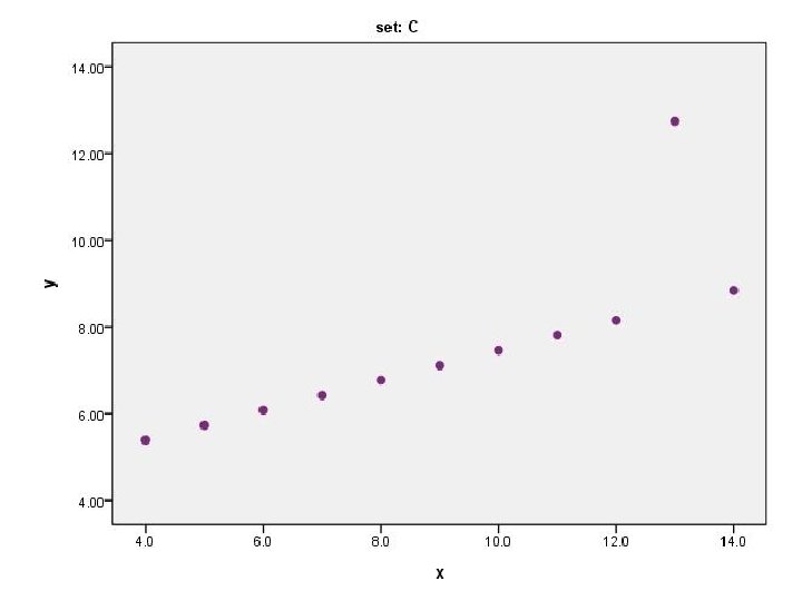
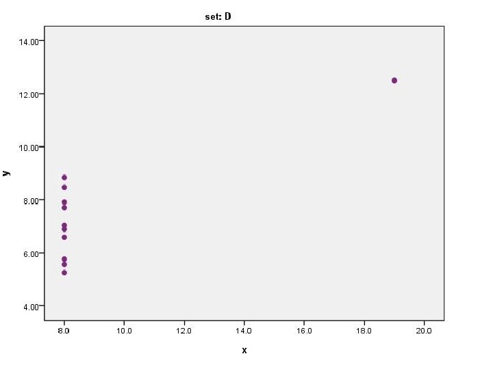
Why You Need Inspect Scatterplots • Data are at http: //core. ecu. edu/psyc/wuenschk/SPSS/ Corr_Regr. sav • Four sets of bivariate data. • Bring into SPSS and Split File by “set. ”

Predict Y from X in Four Different Data Sets