Chapter 4 Regression Regression Like correlation regression addresses

Chapter 4 Regression

Regression • Like correlation, regression addresses linear relationships between quantitative variables X & Y • Objective of correlation quantify direction and strength of linear association • Objective of regression derive best fitting line that describes the association • We are especially interested in the slope of the line

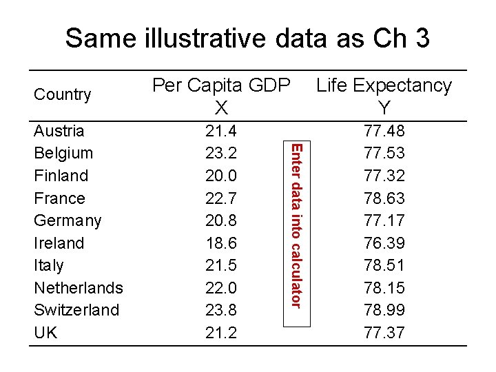
Same illustrative data as Ch 3 Country Life Expectancy Y 21. 4 23. 2 20. 0 22. 7 20. 8 18. 6 21. 5 22. 0 23. 8 21. 2 77. 48 77. 53 77. 32 78. 63 77. 17 76. 39 78. 51 78. 15 78. 99 77. 37 Enter data into calculator Austria Belgium Finland France Germany Ireland Italy Netherlands Switzerland UK Per Capita GDP X

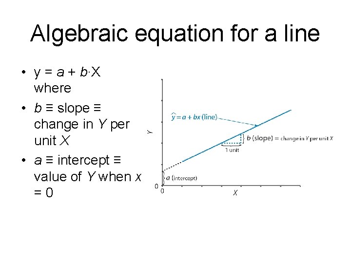
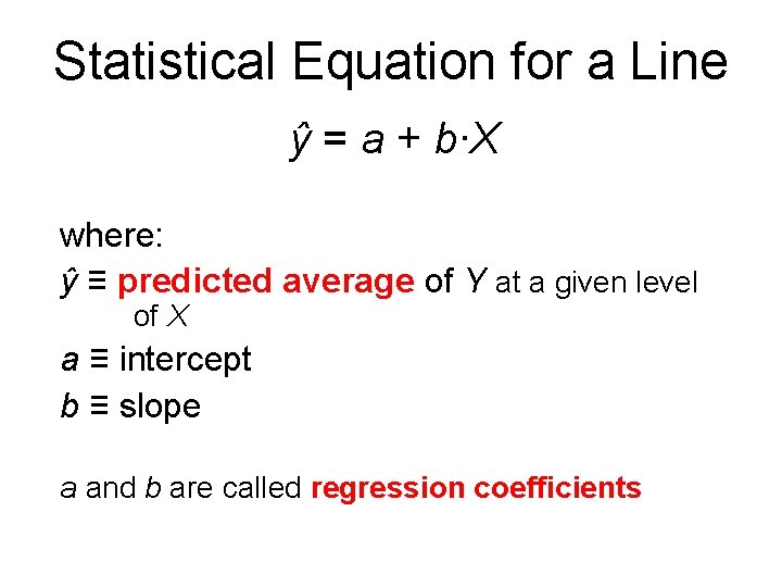
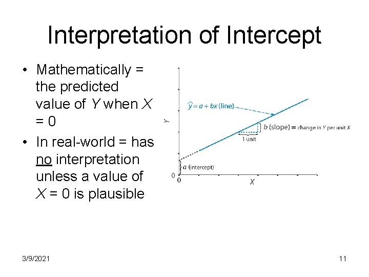
Algebraic equation for a line • y = a + b∙X where • b ≡ slope ≡ change in Y per unit X • a ≡ intercept ≡ value of Y when x =0

Statistical Equation for a Line ŷ = a + b∙X where: ŷ ≡ predicted average of Y at a given level of X a ≡ intercept b ≡ slope a and b are called regression coefficients

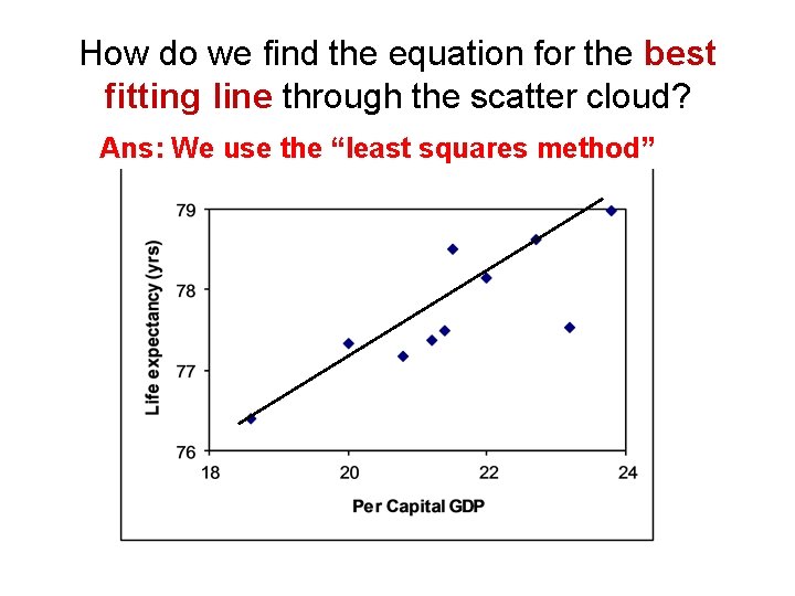
How do we find the equation for the best fitting line through the scatter cloud? Ans: We use the “least squares method”

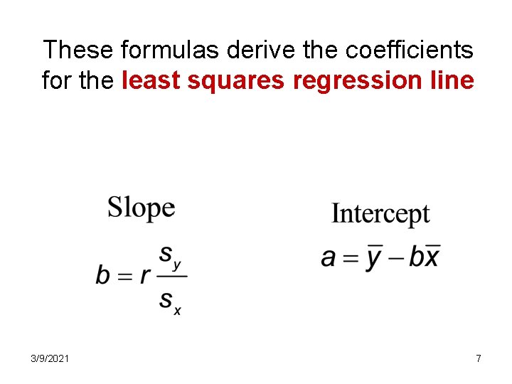
These formulas derive the coefficients for the least squares regression line 3/9/2021 7

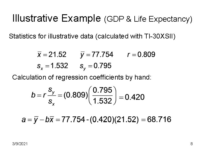
Illustrative Example (GDP & Life Expectancy) Statistics for illustrative data (calculated with TI-30 XSII) Calculation of regression coefficients by hand: 3/9/2021 8

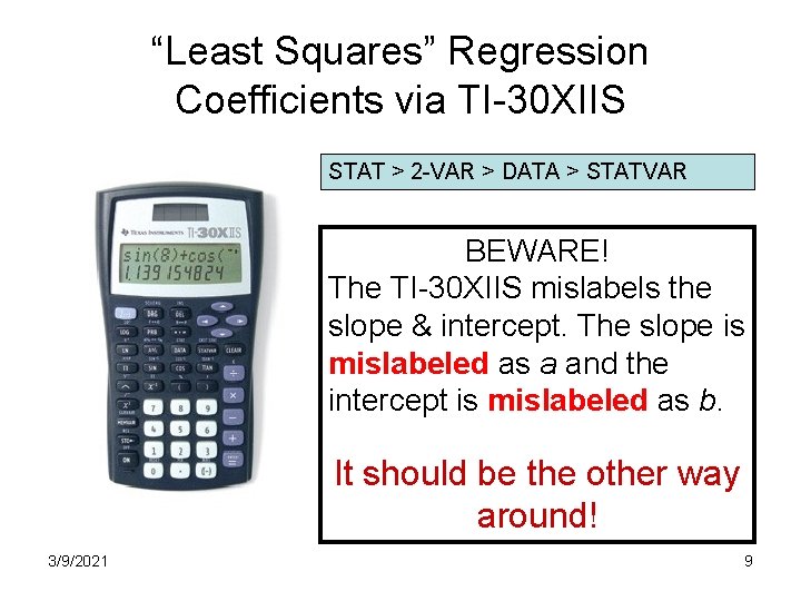
“Least Squares” Regression Coefficients via TI-30 XIIS STAT > 2 -VAR > DATA > STATVAR BEWARE! The TI-30 XIIS mislabels the slope & intercept. The slope is mislabeled as a and the intercept is mislabeled as b. It should be the other way around! 3/9/2021 9

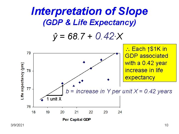
Interpretation of Slope (GDP & Life Expectancy) ŷ = 68. 7 + 0. 42∙X Each ↑$1 K in GDP associated with a 0. 42 year increase in life expectancy b = increase in Y per unit X = 0. 42 years 1 unit X 3/9/2021 10

Interpretation of Intercept • Mathematically = the predicted value of Y when X =0 • In real-world = has no interpretation unless a value of X = 0 is plausible 3/9/2021 11

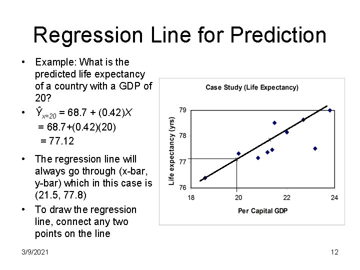
Regression Line for Prediction • Example: What is the predicted life expectancy of a country with a GDP of 20? • Ŷx=20 = 68. 7 + (0. 42)X = 68. 7+(0. 42)(20) = 77. 12 • The regression line will always go through (x-bar, y-bar) which in this case is (21. 5, 77. 8) • To draw the regression line, connect any two points on the line 3/9/2021 x x 12

2 Coefficient of Determination r Interpretation: proportion of the variability in Y mathematically explained by X Our example r =. 809 r 2 =. 8092 = 0. 66. Interpretation: 66% of the variability in Y (life expectancy) mathematically explained* by X (GDP) * mathematically explained ≠ causally explained 3/9/2021 13

Cautions about linear regression 1. Applies to linear relationships only 2. Strongly influenced by outliers, especially when outlier is in the X direction 3. Do not extrapolate! 4. Association ≠ causation (Beware of lurking variables. ) 3/9/2021 14

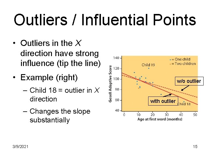
Outliers / Influential Points • Outliers in the X direction have strong influence (tip the line) • Example (right) – Child 18 = outlier in X direction w/o outlier with outlier – Changes the slope substantially 3/9/2021 15

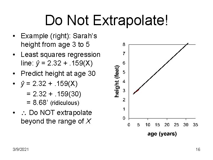
Do Not Extrapolate! • Example (right): Sarah’s height from age 3 to 5 • Least squares regression line: ŷ = 2. 32 +. 159(X) • Predict height at age 30 • ŷ = 2. 32 +. 159(X) = 2. 32 +. 159(30) = 8. 68’ (ridiculous) • Do NOT extrapolate beyond the range of X 3/9/2021 16

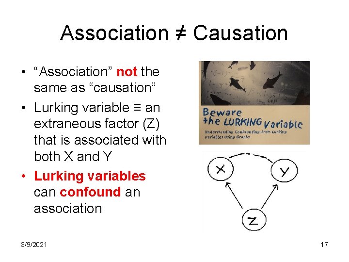
Association ≠ Causation • “Association” not the same as “causation” • Lurking variable ≡ an extraneous factor (Z) that is associated with both X and Y • Lurking variables can confound an association 3/9/2021 17

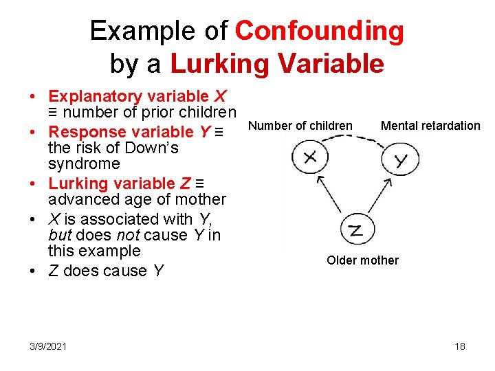
Example of Confounding by a Lurking Variable • Explanatory variable X ≡ number of prior children • Response variable Y ≡ the risk of Down’s syndrome • Lurking variable Z ≡ advanced age of mother • X is associated with Y, but does not cause Y in this example • Z does cause Y 3/9/2021 Number of children Mental retardation Older mother 18

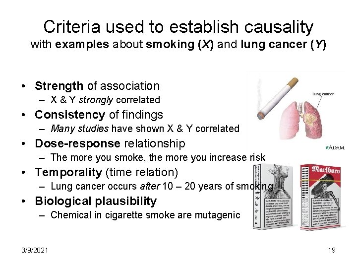
Criteria used to establish causality with examples about smoking (X) and lung cancer (Y) • Strength of association – X & Y strongly correlated • Consistency of findings – Many studies have shown X & Y correlated • Dose-response relationship – The more you smoke, the more you increase risk • Temporality (time relation) – Lung cancer occurs after 10 – 20 years of smoking • Biological plausibility – Chemical in cigarette smoke are mutagenic 3/9/2021 19