136 Chapter 4 Higher Order Differential Equations Highest

136 Chapter 4 Higher Order Differential Equations Highest differentiation: , n > 1 Most of the methods in Chapter 4 are applied for the linear DE.

137 附錄四 DE 的分類 Homogeneous Constant coefficients Linear Cauchy-Euler DE Nonhomogeneous Homogeneous Nonhomogeneous Others Nonlinear Homogeneous Nonhomogeneous

附錄五 Higher Order DE 解法 linear homogeneous particular solution multiple linear DEs reduction of order nonlinear reduction of order auxiliary function Cauchy-Euler “guess” method annihilator variation of parameters elimination method Taylor series numerical method both (but mainly linear) series solution transform Laplace transform Fourier series Fourier cosine series Fourier transform 138

4 -1 Linear Differential Equations: Basic Theory 4. 1. 1 Initial-Value and Boundary Value Problems 4. 1. 1. 1 The nth Order Initial Value Problem i. e. , the nth order linear DE with the constraints at the same point …………. . ………………. . n initial conditions 139

140 Theorem 4. 1. 1 For an interval I that contains the point x 0 If a 0(x), a 1(x), a 2(x), ……. , an − 1(x ), an(x) are continuous at x = x 0 an(x 0) 0 (很像Section 2 -3 當中沒有 singular point 的條件) then for the problem on page 139, the solution y(x) exists and is unique on the interval I that contains the point x 0 (Interval I 的範圍，取決於何時 an(x) = 0 以及 何時 ak(x) (k = 0 ~ n) 不為continuous) Otherwise, the solution is either non-unique or does not exist. (infinite number of solutions) (no solution)

141 Example 1 (text page 119) Example 2 (text page 120) 有無限多組解 c 為任意之常數

142 比較： There is only one solution x (0, ) Note: The initial value can also be the form as: (general initial condition)

4. 1. 1. 2 nth Order Boundary Value Problem Boundary conditions are specified at different points 比較：Initial conditions are specified at the same points 例子： subject to 或 或 An nth order linear DE with n boundary conditions may have a unique solution, no solution, or infinite number of solutions. 143

144 Example 3 (text page 120) solution: (1) (2) c 2 is any constant (infinite number of solutions) (unique solution)

4. 1. 2 Homogeneous Equations 4. 1. 2. 1 Definition g(x) = 0 homogeneous g(x) 0 nonhomogeneous 重要名詞：Associated homogeneous equation The associated homogeneous equation of a nonhomogeneous DE: Setting g(x) = 0 • Review: Section 2 -3, pages 53, 55 145

146 4. 1. 2. 2 New Notations Notation: 可改寫成 可再改寫成

147 4. 1. 2. 3 Solution of the Homogeneous Equation [Theorem 4. 1. 5] For an nth order homogeneous linear DE L(y) = 0, if y 1(t), y 2(t), …. . , yn(t) are the solutions of L(y) = 0 y 1(t), y 2(t), …. . , yn(t) are linearly independent then any solution of the homogeneous linear DE can be expressed as: 可以和矩陣的概念相比較

148 From Theorem 4. 1. 5: An nth order homogeneous linear DE has n linearly independent solutions. Find n linearly independent solutions == Find all the solutions of an nth order homogeneous linear DE y 1(t), y 2(t), …. . , yn(t): fundamental set of solutions : general solution of the homogenous linear DE (又稱做 complementary function) 也是重要名詞

149 Definition 4. 1 Linear Dependence / Independence If there is no solution other than c 1 = c 2 = ……. = cn = 0 for the following equality then y 1(t), y 2(t), …. . , yn(t) are said to be linearly independent. Otherwise, they are linearly dependent. 判斷是否為 linearly independent 的方法: Wronskian

150 Definition 4. 2 Wronskian linearly independent

151 4. 1. 2. 4 Examples Example 9 (text page 127) y 1 = ex, y 2 = e 2 x, and y 3 = e 3 x are three of the solutions Since Therefore, y 1, y 2, and y 3 are linear independent for any x general solution: x (− , )

4. 1. 3 Nonhomogeneous Equations (可和 page 55 相比較) 152 Nonhomogeneous linear DE Part 1 Associated homogeneous DE Part 2 particular solution (any solution of the nonhomogeneous linear DE) find n linearly independent solutions general solution of the nonhomogeneous linear DE

153 Theorem 4. 1. 6 general solution of a nonhomogeneous linear DE general solution of the associated homogeneous function (complementary function) particular solution (any solution) of the nonhomogeneous linear DE general solution of the nonhomogeneous linear DE

154 Example 10 (text page 128) Particular solution Three linearly independent solution , Check by Wronskian (Example 9) General solution:

Theorem 4. 1. 7 Superposition Principle If is the particular solution of : is the particular solution of then is the particular solution of 155

Example 11 (text page 129) is a particular solution of is a particular solution of 156

4. 1. 4 名詞 157 initial conditions, boundary conditions (pages 139, 143) (重要名詞) associated homogeneous equation , complementary function (page 145) (重要名詞) fundamental set of solutions (page 148) Wronskian (page 150) particular solution (page 152) general solution of the homogenous linear DE (page 148) general solution of the nonhomogenous linear DE (page 152)

158 4. 1. 5 本節要注意的地方 (1) Most of theories in Section 4. 1 are applied to the linear DE (2) 注意 initial conditions 和 boundary conditions 之間的不同 (3) 快速判斷 linear independent

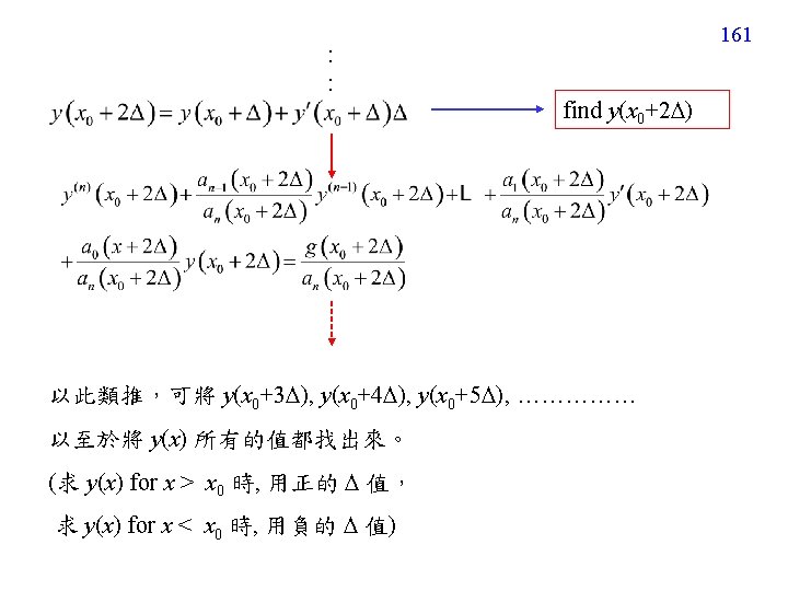
159 (補充 1) Theorem 4. 1. 1 的解釋 ………………. . When an(x 0) 0 find y(n)(x 0) find y(n− 1)(x 0+ ) (根據 , )

160 以此類推 find y(n− 2)(x 0+ ) find y(n− 3)(x 0+ ) : : find y(x 0+ ) find y(n)(x 0+ ) find y(n− 1)(x 0+2 ) find y(n− 2)(x 0+2 )

162 Requirement 1: a 0(x), a 1(x), a 2(x), ……. , an − 1(x ), an(x) are continuous 是為了讓 ak(x 0+m ) 皆可以定義 Requirement 2: an(x) 0 是為了讓 ak(x 0+m ) /an(x 0+m ) 不為無限 大

4 -2 Reduction of Order 4. 2. 1 適用情形 (1) (2) (3) Suitable for the 2 nd order linear homogeneous DE (4) One of the nontrivial solution y 1(x) has been known. 163

164 4. 2. 2 解法 假設 先將DE 變成 Standard form If y(x) = u(x) y 1(x) , zero (比較 Section 2 -3)

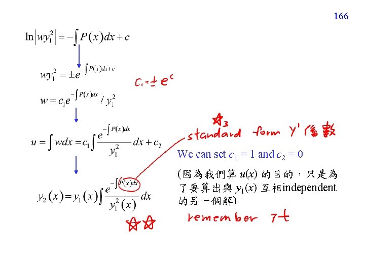
set w = u' multiplied by dx/(y 1 w) separable variable (with 3 variables) 165

4. 2. 3 例子 Example 1 (text page 132) We have known that y 1 = ex is one of the solution P(x) = 0 Specially, set c = – 2, (y 2(x) 只要 independent of y 1(x) 即可 所以 c 的值可以任意設) General solution: 167

168 Example 2 (text page 133) (將課本 x 的範圍做更改 ) when x (− , 0) We have known that y 1 = x 2 is one of the solution Note: the interval of x If x (0, ) (x > 0), 如課本 If x < 0,

170 附錄六： Hyperbolic Function 比較：

171

172

173

附錄七 Linear DE 解法的步驟 (參照講義 page 152) 174 Step 1: Find the general solution (i. e. , the complementary function ) of the associated homogeneous DE (Sections 4 -2, 4 -3, 4 -7) Step 2: Find the particular solution (Sections 4 -4, 4 -5, 4 -6) Step 3: Combine the complementary function and the particular solution Extra Step: Consider the initial (or boundary) conditions

4 -3 Homogeneous Linear Equations with Constant Coefficients 本節使用 auxiliary equation 的方法來解 homogeneous DE KK: [ ] 4 -3 -1 限制條件: (1) homogeneous (2) linear (3) constant coefficients a 0, a 1, a 2, …. , an are constants (the simplest case of the higher order DEs) 175

4 -3 -2 解法 解法核心： Suppose that the solutions has the form of emx Example: y''(x) 3 y'(x) + 2 y(x) = 0 Set y(x) = emx, m 2 emx 3 m emx + 2 emx = 0 m 2 3 m + 2 = 0 solve m 可以直接把 n 次微分用 mn 取代，變成一個多項式 這個多項式被稱為 auxiliary equation 176

177 解法流程 Step 1 -1 auxiliary function Step 1 -1 Find n roots , m 1, m 2, m 3, …. , mn (If m 1, m 2, m 3, …. , mn are distinct) Step 1 -2 n linearly independent solutions (有三個 Cases) Step 1 -3 Complementary function

4 -3 -3 Three Cases for Roots (2 nd Order DE) 178 roots solutions Case 1 m 1 m 2, m 1, m 2 are real (其實 m 1, m 2 不必限制為 real)

Case 2 m 1 = m 2 (m 1 and m 2 are of course real) First solution: Second solution: using the method of “Reduction of Order” 179

Case 3 m 1 m 2 , m 1 and m 2 are conjugate and complex Solution: Another form: set c 1 = C 1 + C 2 and c 2 = j. C 1 − j. C 2 c 1 and c 2 are some constant 180

181 Example 1 (text page 137) (a) 2 m 2 − 5 m − 3 = 0, m 1 = − 1/2, m 2 = 3 (b) m 2 − 10 m + 25 = 0, m 1 = 5, m 2 = 5 (c) m 2 + 4 m + 7 = 0,

4 -3 -4 Three + 1 Cases for Roots (Higher Order DE) 182 For higher order case auxiliary function: roots: m 1, m 2, m 3, …. , mn (1) If mp mq for p = 1, 2, …, n and p q (也就是這個多項式在 mq 的地方只有一個根) then is a solution of the DE. 重覆次數 (2) If the multiplicities of mq is k (當這個多項式在 mq 的地方有 k 個根), are the solutions of the DE.

(3) If both + j and − j are the roots of the auxiliary function, 183 then are the solutions of the DE. (4) If the multiplicities of + j is k and the multiplicities of − j is also k，then are the solutions of the DE.

184 Note: If + j is a root of a real coefficient polynomial, then − j is also a root of the polynomial. a 0, a 1, a 2, …. , an are real

185 Example 3 (text page 138) Solve Step 1 -1 m 1 = 1, m 2 = m 3 = 2 Step 1 -2 3 independent solutions: Step 1 -3 general solution:

Example 4 (text page 138) Solve Step 1 -1 four roots: i, i, i Step 1 -2 4 independent solutions: Step 1 -3 general solution: 186

4 -3 -5 How to Find the Roots 187 (1) Formulas Solutions: (太複雜了 )

188 (2) Observing 例如： 1 是否為 root 看係數和是否為 0 又如： factor: 1, 3 factor: 1, 2, 4 possible roots: 1, 2, 4, 1/3, 2/3, 4/3 test for each possible root find that 1/3 is indeed a root

189 (3) Solving the roots of a polynomial by software Maple Mathematica (by the commands of Nsolve and Find. Root) Matlab ( by the command of roots)

191 練習題 Sec. 4 -1: 3, 7, 8, 10, 13, 20, 24, 29, 33, 36 Sec. 4 -2: 2, 4, 9, 13, 14, 16, 18, 19 Sec. 4 -3: 7, 16, 20, 22, 24, 28, 33, 39, 41, 52, 54, 56, 59, 61, 63

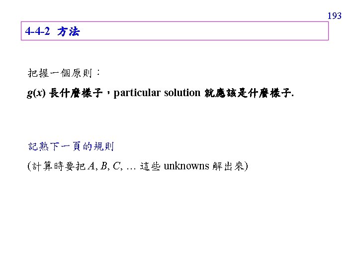
192 4 -4 Undetermined Coefficients – Superposition Approach This section introduces some method of “guessing” the particular solution. 4 -4 -1 方法適用條件 (1) (2) Suitable for linear and constant coefficient DE. (3) g(x), g'(x), g'' (x), g'''(x), g(4)(x), g(5)(x), ………contain finite number of terms.

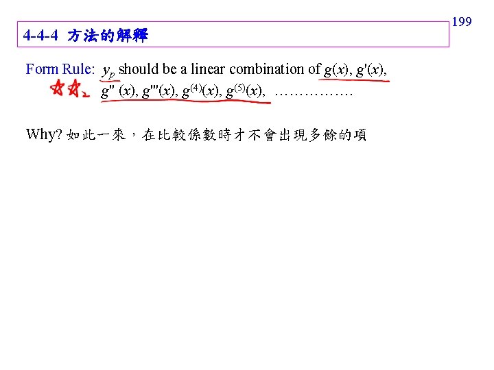
194 Trial Particular Solutions (from text page 146) g(x) Form of yp 1 (any constant) A 5 x + 7 Ax + B 3 x 2 – 2 Ax 2 + Bx + C x 3 – x + 1 Ax 3 + Bx 2 + Cx + E sin 4 x Acos 4 x + Bsin 4 x cos 4 x Acos 4 x + Bsin 4 x e 5 x Ae 5 x (9 x – 2)e 5 x (Ax + B)e 5 x x 2 e 5 x (Ax 2 + Bx + C)e 5 x e 3 xsin 4 x Ae 3 xcos 4 x + Be 3 xsin 4 x 5 x 2 sin 4 x (Ax 2 + Bx + C)cos 4 x + (Ex 2 + Fx + G)sin 4 x xe 3 xcos 4 x (Ax + B)e 3 xcos 4 x + (Cx + E)e 3 xsin 4 x It comes from the “form rule”. See page 199.

195 yp = ?

196 4 -4 -3 Examples Example 2 (text page 144) Step 1: find the solution of the associated homogeneous equation Guess Step 2: particular solution A = 6/73, B = 16/73 Step 3: General solution:

Example 3 (text page 145) Step 1: Find the solution of Step 2: Particular solution guess 197

Particular solution Step 3: General solution 198

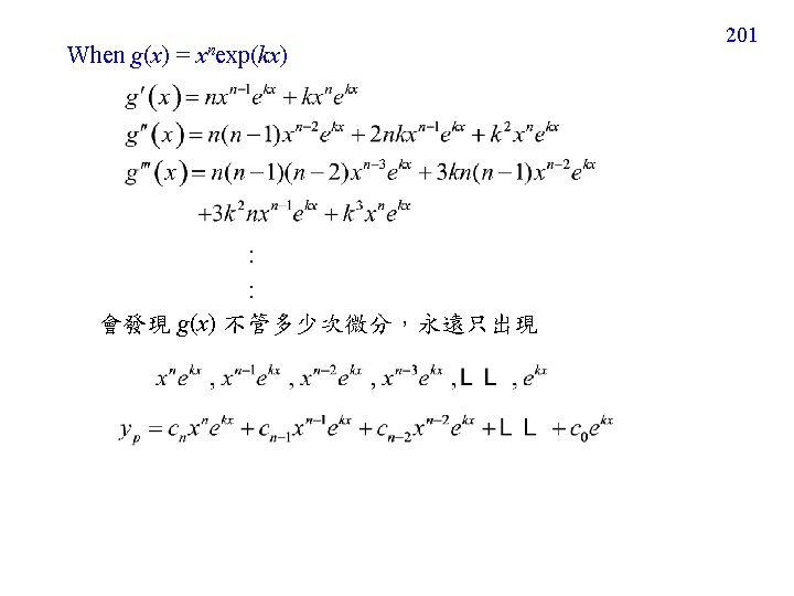
When g(x) = xn When g(x) = cos kx When g(x) = exp(kx) 200

202 4 -4 -5 Glitch of the method: Example 4 (text page 146) Particular solution guessed by Form Rule: (no solution) Why?

203 Glitch condition 1: The particular solution we guess belongs to the complementary function. For Example 4 Complementary function 解決方法：再乘一個 x

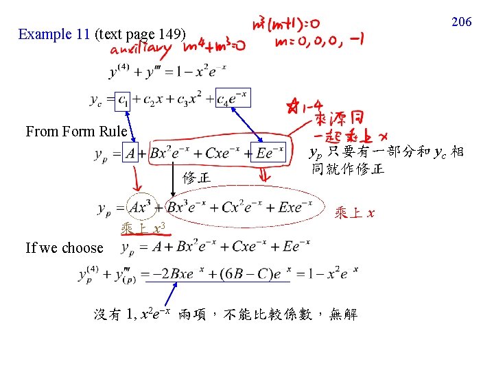
204 Example 7 (text page 148) From Form Rule, the particular solution is Aex 如果乘一個 x 不夠，則再乘一個 x

205 Example 8 (text page 148) Step 1 Step 2 注意： sinx, cosx 都要 乘上 x Step 3 Step 4 Solving c 1 and c 2 by initial conditions (最後才解 IVP)

207 If we choose 沒有 x 2 e x 這一項，不能比較係數，無解 If we choose A = 1/6, B = 1/3, C = 3, E = 12

208 Glitch condition 2: g(x), g'(x), g'' (x), g'''(x), g(4)(x), g(5)(x), …………… contain infinite number of terms. If g(x) = ln x If g(x) = exp(x 2) : :

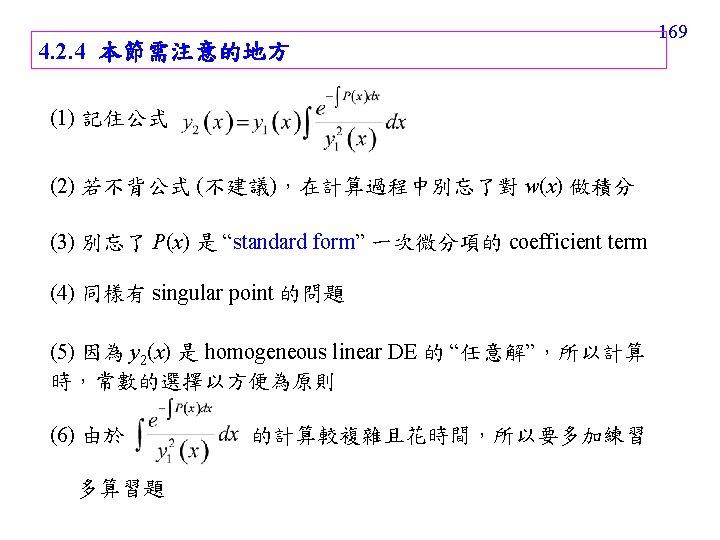
209 4 -4 -6 本節需要注意的地方 (1) 記住 Table 4. 1 的 particular solution 的假設方法 (其實和 “form rule” 有相密切的關聯) (2) 注意 “glitch condition” 另外，“同一類” 的 term 要乘上相同的東西 (參考 Example 11) (3) 所以要先算 complementary function，再算 particular solution (4) 同樣的方法，也可以用在 1 st order 的情形 (5) 本方法只適用於 linear, constant coefficient DE

210 4 -5 Undetermined Coefficients – Annihilator Approach For a linear DE: Annihilator Operator: 能夠「殲滅」 g(x) 的 operator 4 -5 -1 方法適用條件 (1) Linear， (2) Constant coefficients (3) g(x), g'(x), g'' (x), g'''(x), g(4)(x), g(5)(x), ………contain finite number of terms.

211 4 -5 -2 Find the Annihilator Example 1: (text page 153) annihilator: D 4 annihilator: D + 3

212 annihilator: (D − 2)2 = D 2 − 4 D + 4 註：當各個微分項的 coefficients 皆為 constants 時，function of D 的計算方式和 function of x 的計算方式相同 (x − 2)2 = x 2 − 4 x + 4 (D − 2)2 = D 2 − 4 D + 4

213 General rule 1: If then the annihilator is 注意： annihilator 和 a 0, a 1, …… , an 無關 只和 , n 有關 The annihilator is independent of the constant multiplied in the front of each term.

General rule 2: If b 1 0 or b 2 0 then the annihilator is Example 2: (text page 154) annihilator Example 5: (text page 156) annihilator Example 6: (text page 157) annihilator 214

General rule 3: If g(x) = g 1(x) + g 2(x) + …… + gk(x) Lh[gh(x)] = 0 but Lh[gm(x)] 0 if m h, then the annihilator of g(x) is the product of Lh (h = 1 ~ k) Proof: (因為 L 1, L 2 為 linear DE with constant coefficient, L 1 L 2 = L 2 L 1 ) 215

216 Similarly, : : Therefore,

217 Example 7 (text page 157) annihilator: D 3 annihilator: D − 5 annihilator: (D − 2)3 annihilator of g(x): D 3 (D − 2)3 (D − 5)

218 4 -5 -3 Using the Annihilator to Find the Particular Solution Step 2 -1 Find the annihilator L 1 of g(x) Step 2 -2 如果原來的 linear & constant coefficient DE 是 那麼將 DE 變成如下的型態： (homogeneous linear & constant coefficient DE) 註： If then

219 Step 2 -3 Use the method in Section 4 -3 to find the solution of Step 2 -4 Find the particular solution. The particular solution yp is a solution of but not a solution of (Proof): Since , if g(x) 0, should be nonzero. Moreover, . Step 2 -5 Solve the unknowns

220 solutions of particular solution yp solutions of 本節核心概念 solutions of

4 -5 -4 Examples 221 Example 3 (text page 155) Step 1: Complementary function (solution of the associated homogeneous function) Step 2 -1: Annihilation: D 3 Step 2 -2: Step 2 -3: auxiliary function roots: m 1 = m 2 = m 3 = 0, m 4 = − 1, m 5 = − 2 移除和 complementary Solution for : function 相同的部分

Step 2 -4: particular solution Step 2 -5: Step 3: 222

Example 4 (text page 156) Step 1: Complementary function From auxiliary function, m 2 − 3 m = 0, roots: 0, 3 Step 2 -1: Find the annihilator D − 3 annihilate but cannot annihilate (D 2 + 1) annihilate but cannot annihilate (D − 3)(D 2 + 1) is the annihilator of Step 2 -2: 223

Step 2 -3: auxiliary function: 224 易犯錯的地方 solution of : Step 2 -4: particular solution 代回原式 並比較係數 Step 2 -5: Step 3: general solution

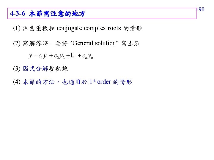
4 -5 -5 本節要注意的地方 (1) 所以要先算 complementary function，再算 particular solution (2) 若有兩個以上的 annihilator，選其中較簡單的即可 (3) 計算 auxiliary function 時有時容易犯錯 (4) 的解和 的解不一樣。 (5) 這方法，只適用於 constant coefficient linear DE (因為，還需借助 auxiliary function) 225

226 The thing that can be done by the annihilator approach can always be done by the “guessing” method in Section 4 -4, too.

227 4 -6 Variation of Parameters 4 -6 -1 方法的限制 The method can solve the particular solution for any linear DE (1) May not have constant coefficients (2) g(x) may not be of the special forms

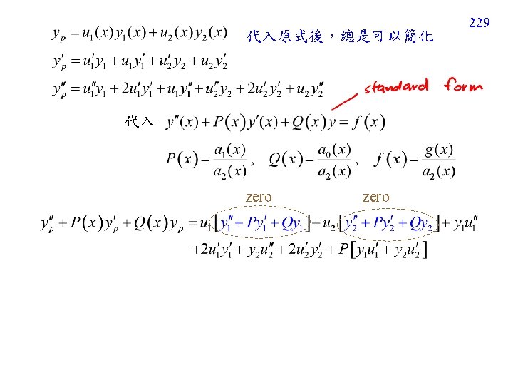
228 4 -6 -2 Case of the 2 nd order linear DE associated homogeneous equation: Suppose that the solution of the associated homogeneous equation is Then the particular solution is assumed as: (方法的基本精神)

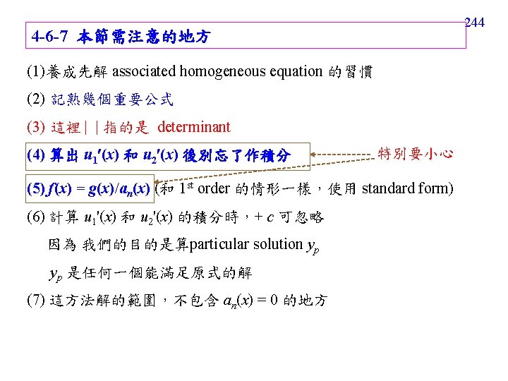
231 where | |: determinant 可以和 1 st order case (page 58) 相比較

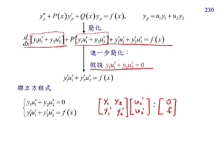
4 -6 -3 Process for the 2 nd Step 2 -1 變成 standard form Step 2 -2 Step 2 -3 Step 2 -4 Step 2 -5 Order Case 232

4 -6 -4 Examples Example 1 (text page 162) Step 1: solution of Step 2 -2: Step 2 -3: 233

Step 2 -4: Step 2 -5: Step 3: 234

235 Example 2 (text page 163) Step 1: solution of Step 2 -1: standard form: Step 2 -2: Step 2 -3: Step 2 -4: (未完待續) 注意 算法

236 Step 2 -5: Step 3: Note: 課本 Interval (0, /6) 應該改為(0, /3)

Example 3 (text page 164) Note: 沒有 analytic 的解 所以直接表示成 (複習 page 45) 237

238 4 -6 -5 Case of the Higher Order Linear DE Solution of the associated homogeneous equation: The particular solution is assumed as:

239

240 Wk: replace the kth column of W by For example, when n = 3,

4 -6 -6 Process of the Higher Order Case Step 2 -1 變成 standard form Step 2 -2 Calculate W, W 1, W 2, …. , Wn (see page 239) Step 2 -3 ……… Step 2 -4 ……. Step 2 -5 241

242 Exercise 26 Complementary function:

243 for - /4 < x < /4 Note: - /4 , /4 are singular points