Chapter 8 Solving Second order differential equations numerically

Chapter 8 Solving Second order differential equations numerically

Online lecture materials • The online lecture notes by Dr. Tai. Ran Hsu of San José State University, http: //www. engr. sjsu. edu/trhsu/Chapt er%204%20 Second%20 order%20 DEs. p df provides a very clear explanation of the solutions and applications of some typical second order differential equations.

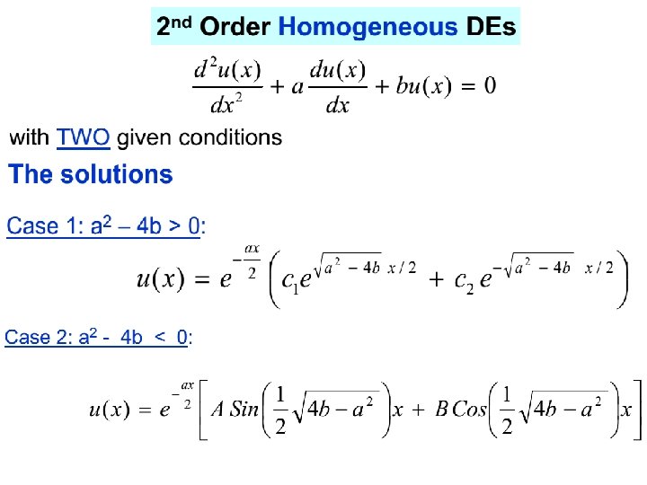
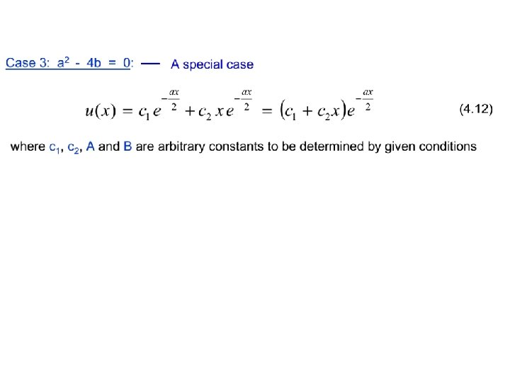
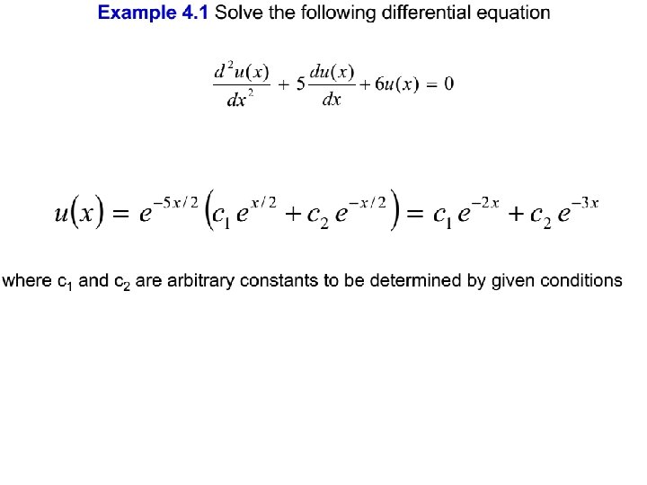
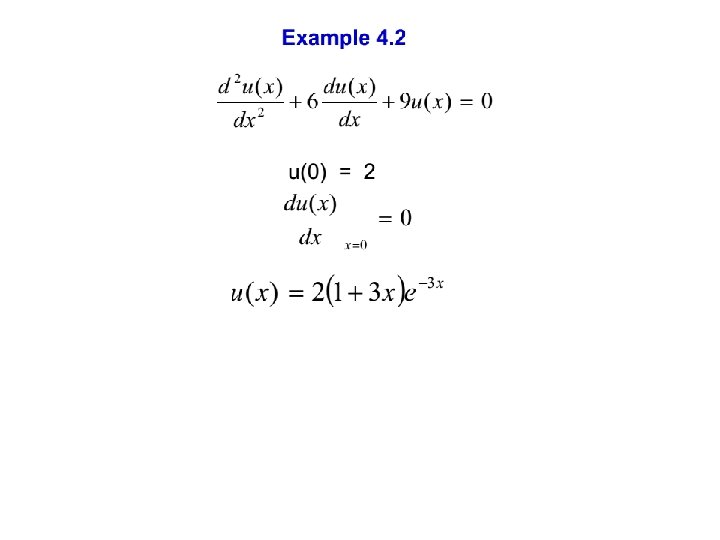
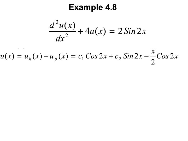
Typical second order, non-homogeneous ordinary differential equations n(x)

Typical second order, non-homogeneous ordinary differential equations n(x)

Guess: After some algebra

Simple Harmonic pendulum as a special case of second order DE Force on the pendulum for small oscillation, Equation of motion (Eo. M) l r n(x) The period of the SHO is given by

Simple Harmonic pendulum as a special case of second order DE (cont. ) n(x)

Simple Harmonic pendulum as a special case of second order DE (cont. ) Analytical solution:

Simple Harmonic pendulum with drag force as a special case of second order DE Drag force on a moving object, fd = - kv For a pendulum, instantaneous velocity v = wl = l (dq/dt) Hence, fd = - kl (dq/dt). l Consider the net force on the forced pendulum along the tangential direction, in the q 0 limit: fd r v mg

Simple Harmonic pendulum with drag force as a special case of second order DE (cont. ) n(x) l fd rr v mg

1. Underdamped regime (small damping). Still oscillate, but amplitude decay slowly over many period before dying totally. Analytical solutions

2. Overdamped regime (very large damping), decay slowly over several period before dying totally. q is dominated by exponential term. Analytical solutions

3. Critically damped regime, intermediate between under- and overdamping case. Analytical solutions

Overdamped Critically damped Underdamped

See C 8_2 ODE_Pendulum. nb where Dsolve[] solves the three cases of a damped pendulum analytically.

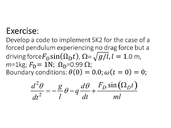
Adding driving force to the damped oscillator: forced oscillator - kl (dq/dt) + FD sin(WDt) WD frequency of the applied force

Analytical solution Resonance happens when

Forced oscillator: An example of non homogeneous 2 nd order DE n(x)

Exercise: Forced oscillator

Second order Runge-Kutta (RK 2) method Consider a generic second order differential equation. It can be numerically solved using second order Runge-Kutta method. Split the second order DE into two first order parts:

Algorithm Set boundary conditions: u(x=x 0)=u 0, u’(x=x 0)=v 0. calculate

Translating the SK 2 algorithm into the case of simple pendulum Set boundary conditions: u(x=x 0)=u 0, u’(x=x 0)=v 0 Set boundary conditions: q(t=t 0)= q 0, q’ (t=t 0)=w 0

Exercise: Develop a code to implement SK 2 for the case of the simple pendulum. Boundary conditions: See C 8_pendulum_RK 2. nb

Translating the SK 2 algorithm into the case of damped pendulum Set boundary conditions: u(x=x 0)=u 0, u’(x=x 0)=v 0 Set boundary conditions: q(t=t 0)= q 0, q’ (t=t 0)=w 0

Sample code: C 8_dampedpendulum_RK 2. nb

Exercise: Stability of the total energy a SHO in RK 2.