Partial Differential Equations All the differential equations involve

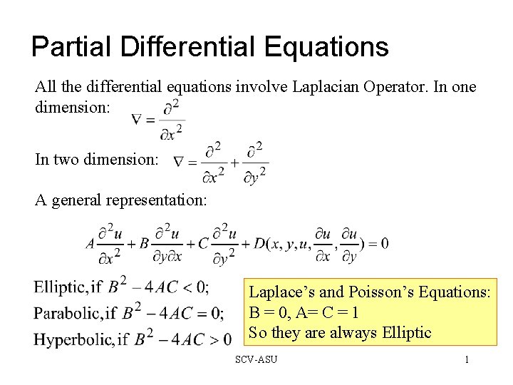
Partial Differential Equations All the differential equations involve Laplacian Operator. In one dimension: In two dimension: A general representation: Laplace’s and Poisson’s Equations: B = 0, A= C = 1 So they are always Elliptic SCV-ASU 1

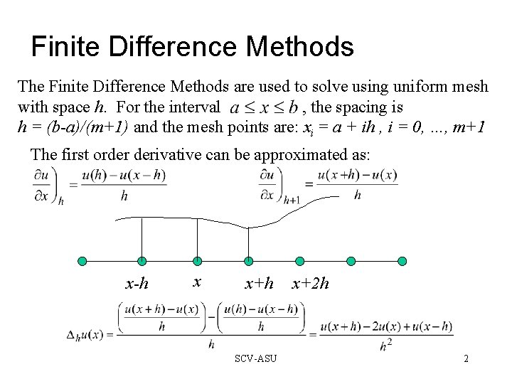
Finite Difference Methods The Finite Difference Methods are used to solve using uniform mesh with space h. For the interval , the spacing is h = (b-a)/(m+1) and the mesh points are: xi = a + ih , i = 0, …, m+1 The first order derivative can be approximated as: x-h x x+h SCV-ASU x+2 h 2

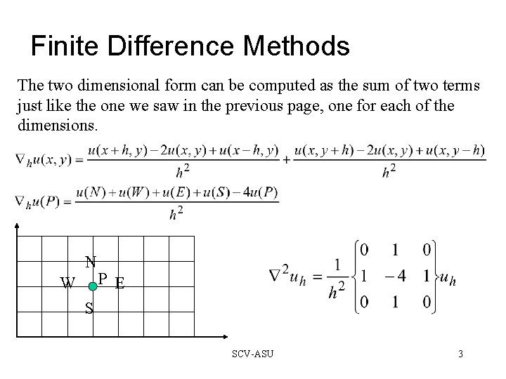
Finite Difference Methods The two dimensional form can be computed as the sum of two terms just like the one we saw in the previous page, one for each of the dimensions. N W P E S SCV-ASU 3

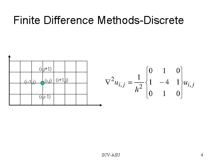
Finite Difference Methods-Discrete (i, j+1) (i-1, j) (i+1, j) (i, j-1) SCV-ASU 4

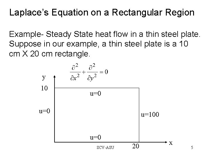
Laplace’s Equation on a Rectangular Region Example- Steady State heat flow in a thin steel plate. Suppose in our example, a thin steel plate is a 10 cm X 20 cm rectangle. y 10 u=0 u=100 u=0 SCV-ASU 20 x 5

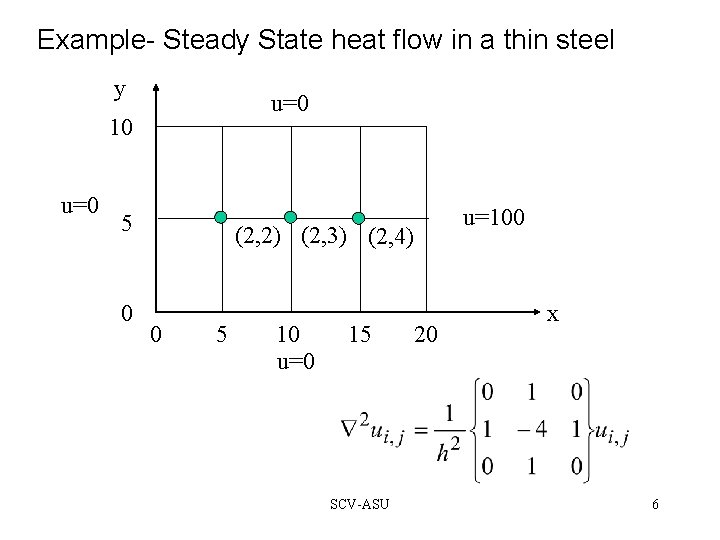
Example- Steady State heat flow in a thin steel y u=0 10 u=0 5 0 (2, 2) (2, 3) (2, 4) 0 5 10 u=0 15 SCV-ASU 20 u=100 x 6

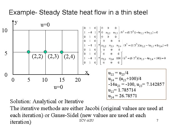
Example- Steady State heat flow in a thin steel y u=0 10 5 0 (2, 2) (2, 3) (2, 4) x 0 5 10 15 u=0 20 u 22 = u 23/4 u 24 = (u 23+100)/4 -14 u 23 = -100, u 23= 7. 142857 u 22= 1. 785714 u 24 = 26. 78571 Solution: Analytical or Iterative The iterative methods are either Jacobi (original values are used at each iteration) or Gauss-Sidel (new values are used at each SCV-ASU 7 iteration)

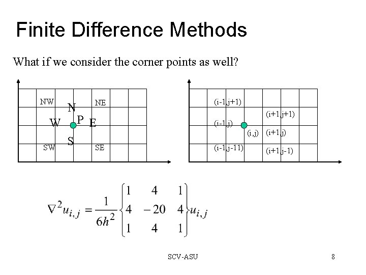
Finite Difference Methods What if we consider the corner points as well? NW N W SW S (i-1, j+1) NE (i+1, j+1) P E (i-1, j) (i+1, j) SE (i-1, j-11) SCV-ASU (i+1, j-1) 8

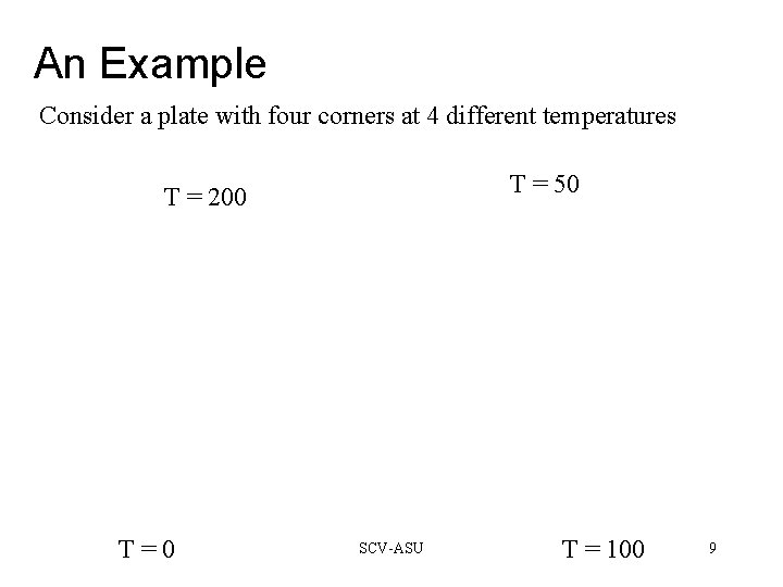
An Example Consider a plate with four corners at 4 different temperatures T = 50 T = 200 T=0 SCV-ASU T = 100 9

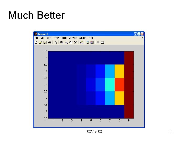
An Example (Misleading) >> x = [0 5 5 0]; >> y = [0 100 50 100]; >> t = [0 100 50 200]; patch(x, y, t, rand(size(t))) SCV-ASU 10

Much Better SCV-ASU 11

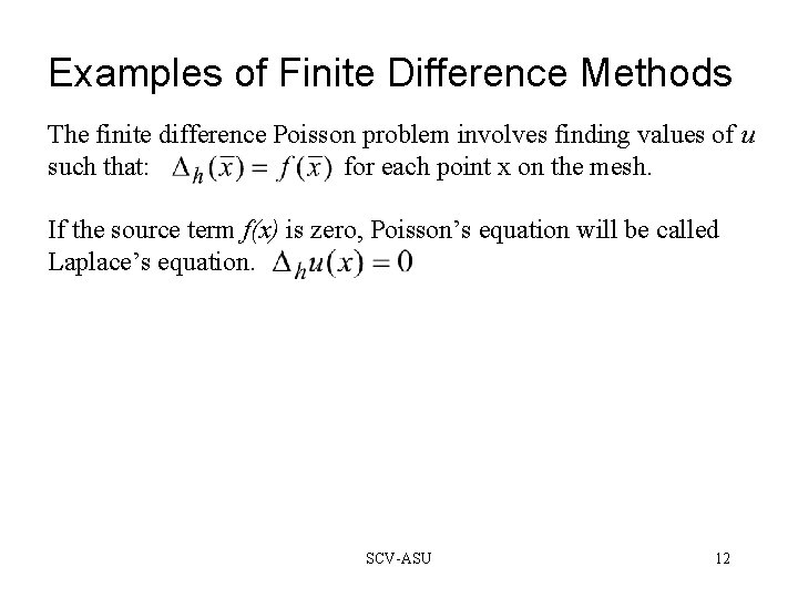
Examples of Finite Difference Methods The finite difference Poisson problem involves finding values of u such that: for each point x on the mesh. If the source term f(x) is zero, Poisson’s equation will be called Laplace’s equation. SCV-ASU 12

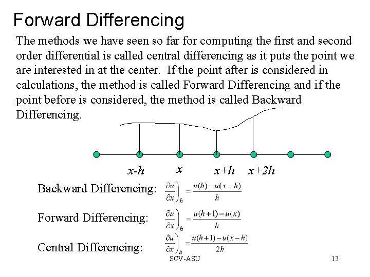
Forward Differencing The methods we have seen so far for computing the first and second order differential is called central differencing as it puts the point we are interested in at the center. If the point after is considered in calculations, the method is called Forward Differencing and if the point before is considered, the method is called Backward Differencing. x-h Backward Differencing: x x+h x+2 h Forward Differencing: Central Differencing: SCV-ASU 13

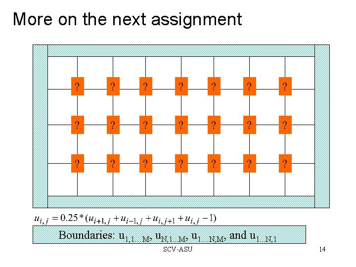
More on the next assignment ? ? ? ? ? ? Boundaries: u 1, 1…M, u. N, 1. . . M, u 1…N, M, and u 1. . . N, 1 SCV-ASU 14