Chapter 8 Solving Second order differential equations numerically

Chapter 8 Solving Second order differential equations numerically

Online lecture materials • The online lecture notes by Dr. Tai. Ran Hsu of San José State University, http: //www. engr. sjsu. edu/trhsu/Chapt er%204%20 Second%20 order%20 DEs. p df provides a very clear explanation of the solutions and applications of some typical second order differential equations.

DSolve • DSolve of Mathematica can provide analytical solution to a generic second order differential equation. See Math_built_in_2 ODE. nb.

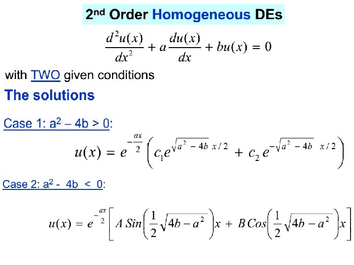
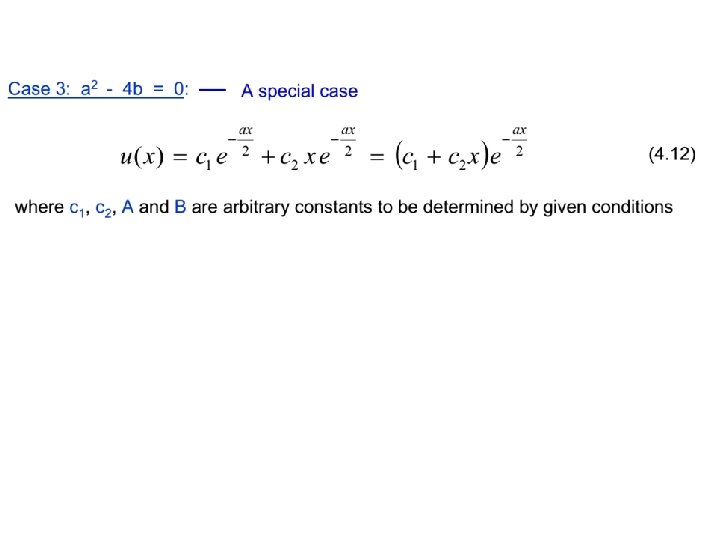
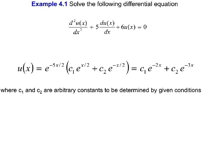
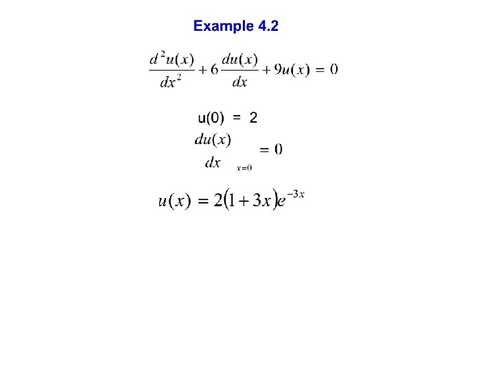
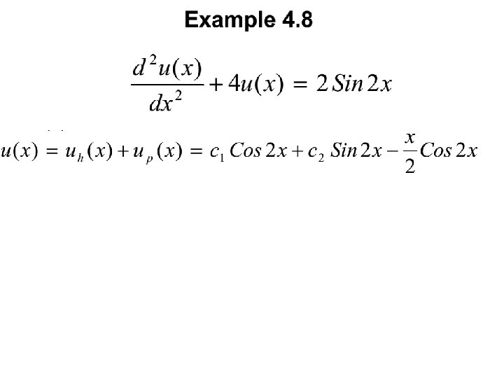
Typical second order, non-homogeneous ordinary differential equations n(x)

Typical second order, non-homogeneous ordinary differential equations n(x)

Guess: After some algebra

Simple Harmonic pendulum as a special case of second order DE Force on the pendulum for small oscillation, Equation of motion (Eo. M) l r n(x) The period of the SHO is given by

Simple Harmonic pendulum as a special case of second order DE (cont. ) n(x)

Simple Harmonic pendulum as a special case of second order DE (cont. ) Analytical solution:

Simple Harmonic pendulum with drag force as a special case of second order DE Drag force on a moving object, fd = - kv For a pendulum, instantaneous velocity v = wl = l (dq/dt) Hence, fd = - kl (dq/dt). l The net force on the forced pendulum along the tangential direction - kl (dq/dt). fd r

Simple Harmonic pendulum with drag force as a special case of second order DE (cont. ) n(x) l fd r

Underdamped regime (small damping). Still oscillate, but amplitude decay slowly over many period before dying totally. Overdamped regime (very large damping), decay slowly over several period before dying totally. q is dominated by exponential term. Analytical solution Critically damped regime, intermediate between under- and overdamping case.

Overdamped Critically damped Underdamped

See 2 ODE_Pendulum. nb where DSolve solves the three cases of a damped pendulum analytically.

Adding driving force to the damped oscillator: forced oscillator - kl (dq/dt) + FD sin(WDt) WD frequency of the applied force

Analytical solution Resonance happens when

Forced oscillator: An example of non homogeneous 2 nd order DE n(x)

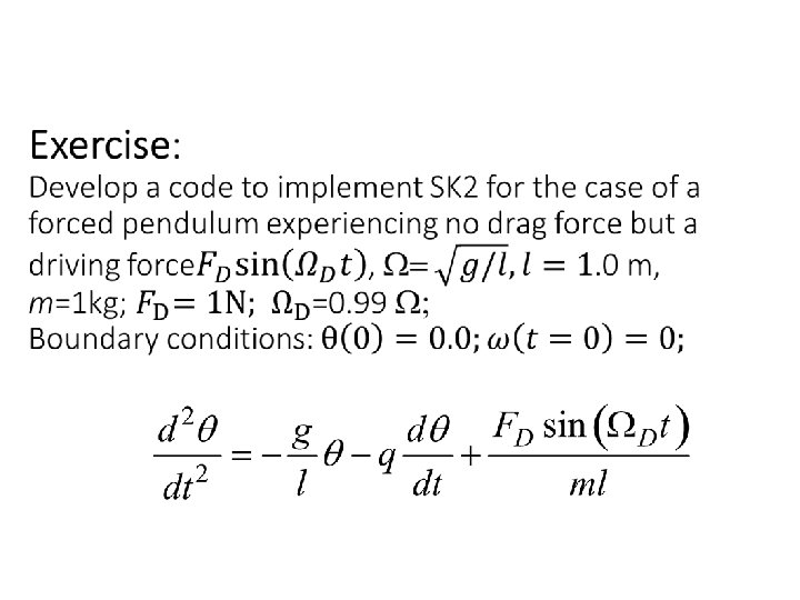
Exercise: Forced oscillator

Second order Runge-Kutta (RK 2) method Consider a generic second order differential equation. It can be numerically solved using second order Runge-Kutta method. First, split the second order DE into two first order parts:

Algorithm Set boundary conditions: u(x=x 0)=u 0, u’(x=x 0)=v 0. calculate

Translating the SK 2 algorithm into the case of simple pendulum Set boundary conditions: u(x=x 0)=u 0, u’(x=x 0)=v 0 Set boundary conditions: q(t=t 0)= q 0, q’ (t=t 0)=w 0

Exercise: Develop a code to implement SK 2 for the case of the simple pendulum. Boundary conditions: See pendulum_RK 2. nb

Translating the SK 2 algorithm into the case of damped pendulum Set boundary conditions: u(x=x 0)=u 0, u’(x=x 0)=v 0 Set boundary conditions: q(t=t 0)= q 0, q’ (t=t 0)=w 0

See pendulum_RK 2. nb

Exercise: Stability of the total energy a SHO in RK 2.