Ordinary Differential Equations and Partial Differential Equations Solutions

Ordinary Differential Equations and Partial Differential Equations: Solutions and Parallelism UCSB CS 240 A Tao Yang Some slides are from K. Yalick/Demmel

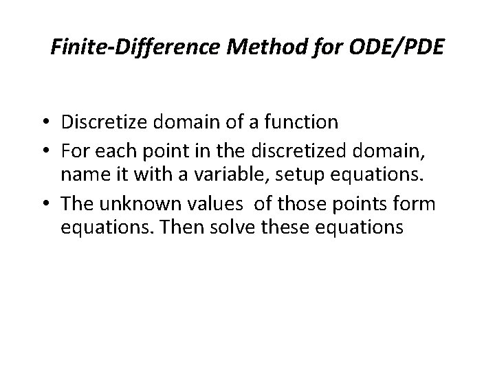
Finite-Difference Method for ODE/PDE • Discretize domain of a function • For each point in the discretized domain, name it with a variable, setup equations. • The unknown values of those points form equations. Then solve these equations

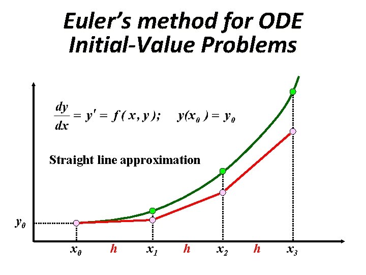
Euler’s method for ODE Initial-Value Problems Straight line approximation y 0 x 0 h x 1 h x 2 h x 3

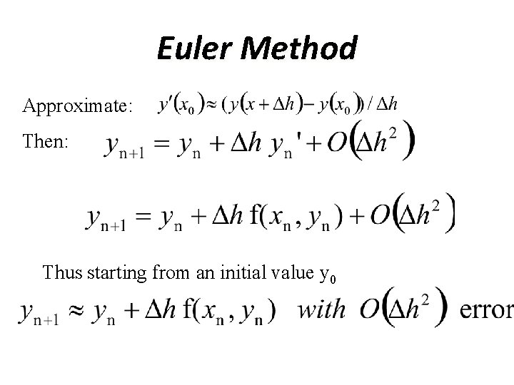
Euler Method Approximate: Then: Thus starting from an initial value y 0

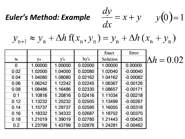
Euler’s Method: Example

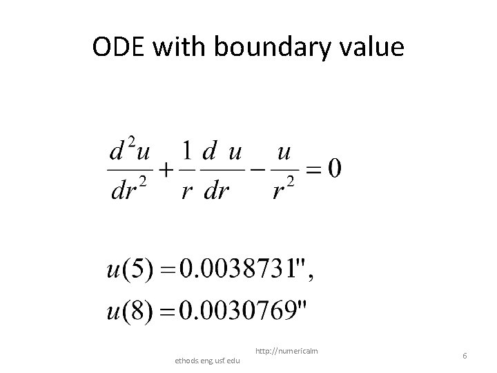
ODE with boundary value ethods. eng. usf. edu http: //numericalm 6

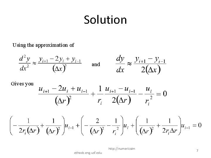
Solution Using the approximation of and Gives you ethods. eng. usf. edu http: //numericalm 7

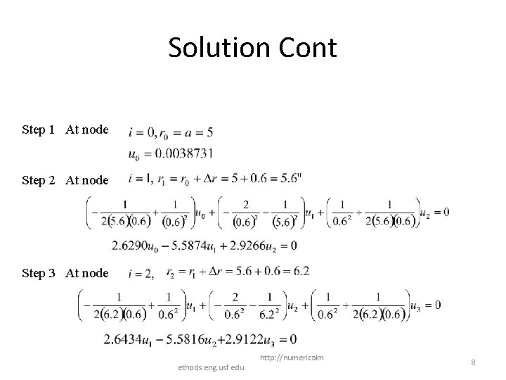
Solution Cont Step 1 At node Step 2 At node Step 3 At node ethods. eng. usf. edu http: //numericalm 8

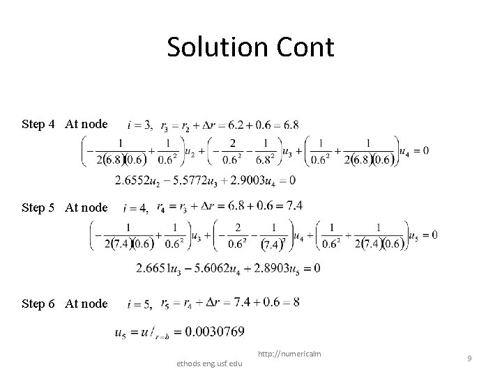
Solution Cont Step 4 At node Step 5 At node Step 6 At node ethods. eng. usf. edu http: //numericalm 9

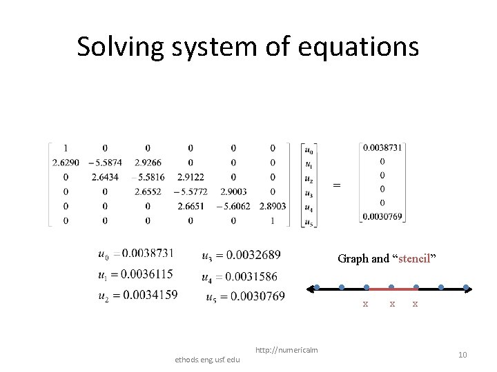
Solving system of equations = Graph and “stencil” x ethods. eng. usf. edu http: //numericalm x x 10

Source: Accelerator Cavity Design Problem (Ko via Husbands)

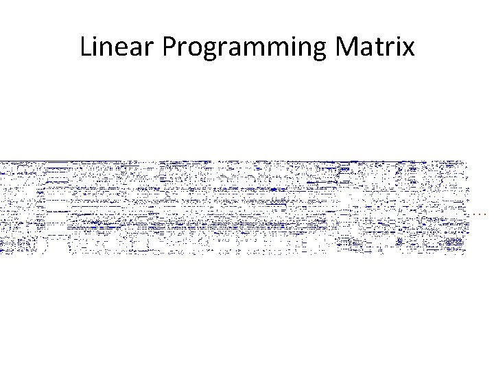
Linear Programming Matrix …

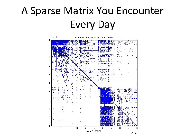
A Sparse Matrix You Encounter Every Day

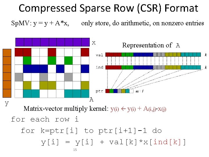
Compressed Sparse Row (CSR) Format Sp. MV: y = y + A*x, only store, do arithmetic, on nonzero entries x y Representation of A A Matrix-vector multiply kernel: y(i) + A(i, j)×x(j) for each row i for k=ptr[i] to ptr[i+1]-1 do y[i] = y[i] + val[k]*x[ind[k]] 15

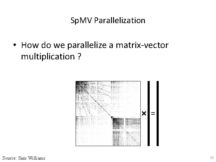
Sp. MV Parallelization • How do we parallelize a matrix-vector multiplication ? Source: Sam Williams 16

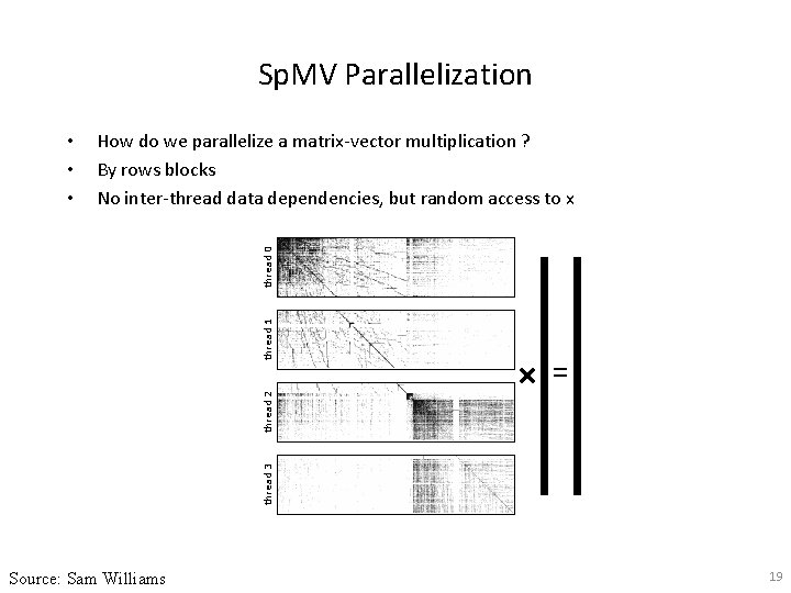
Sp. MV Parallelization How do we parallelize a matrix-vector multiplication ? By rows blocks No inter-thread data dependencies, but random access to x thread 3 thread 2 thread 1 thread 0 • • • Source: Sam Williams 19

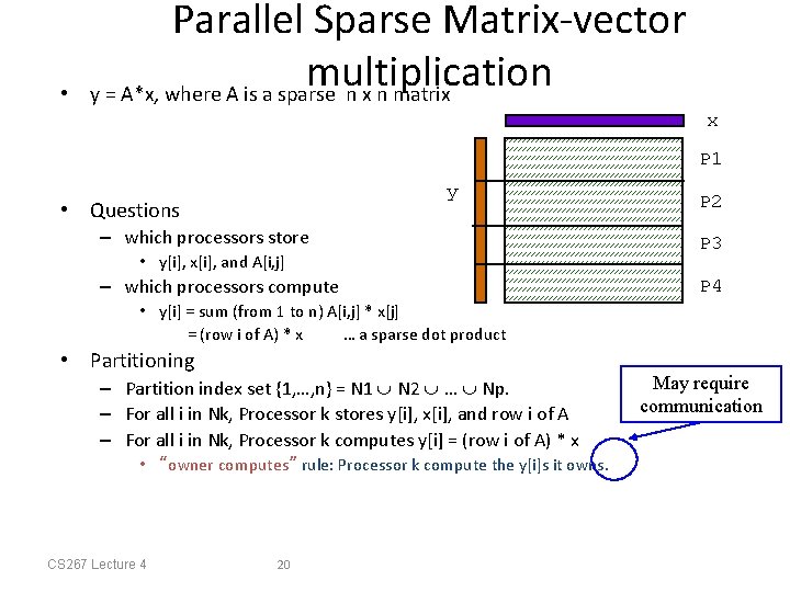
• Parallel Sparse Matrix-vector multiplication y = A*x, where A is a sparse n x n matrix x P 1 y • Questions – which processors store • y[i], x[i], and A[i, j] – which processors compute P 2 P 3 P 4 • y[i] = sum (from 1 to n) A[i, j] * x[j] = (row i of A) * x … a sparse dot product • Partitioning – Partition index set {1, …, n} = N 1 N 2 … Np. – For all i in Nk, Processor k stores y[i], x[i], and row i of A – For all i in Nk, Processor k computes y[i] = (row i of A) * x • “owner computes” rule: Processor k compute the y[i]s it owns. CS 267 Lecture 4 20 May require communication

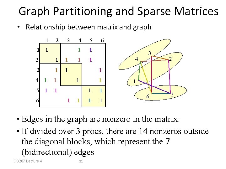
Graph Partitioning and Sparse Matrices • Relationship between matrix and graph 1 1 2 3 1 2 1 1 3 1 1 4 1 1 5 1 1 6 4 5 1 1 4 3 2 1 1 1 6 1 1 1 1 6 5 • Edges in the graph are nonzero in the matrix: • If divided over 3 procs, there are 14 nonzeros outside the diagonal blocks, which represent the 7 (bidirectional) edges CS 267 Lecture 4 21

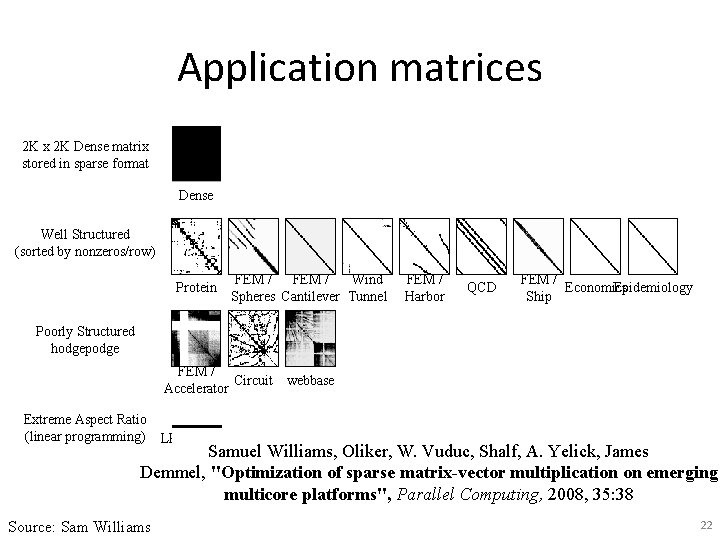
Application matrices 2 K x 2 K Dense matrix stored in sparse format Dense Well Structured (sorted by nonzeros/row) Protein FEM / Wind Spheres Cantilever Tunnel FEM / Harbor QCD FEM / Economics Epidemiology Ship Poorly Structured hodgepodge FEM / Circuit webbase Accelerator Extreme Aspect Ratio (linear programming) LP Samuel Williams, Oliker, W. Vuduc, Shalf, A. Yelick, James Demmel, "Optimization of sparse matrix-vector multiplication on emerging multicore platforms", Parallel Computing, 2008, 35: 38 Source: Sam Williams 22

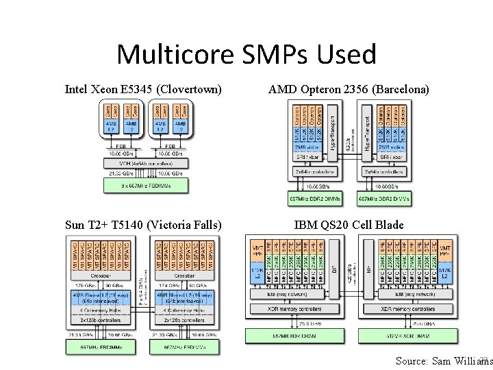
Multicore SMPs Used Intel Xeon E 5345 (Clovertown) AMD Opteron 2356 (Barcelona) Sun T 2+ T 5140 (Victoria Falls) IBM QS 20 Cell Blade 23 Source: Sam Williams

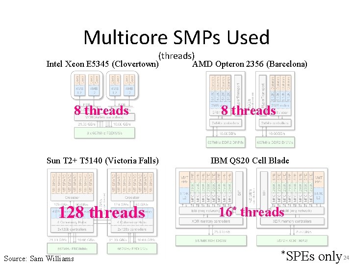
Multicore SMPs Used (threads) Intel Xeon E 5345 (Clovertown) AMD Opteron 2356 (Barcelona) 8 threads Sun T 2+ T 5140 (Victoria Falls) IBM QS 20 Cell Blade 128 threads 16* threads Source: Sam Williams *SPEs only 24

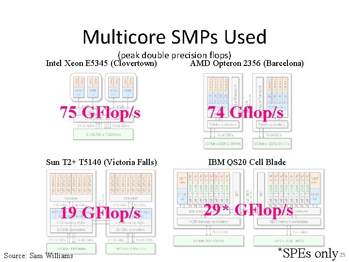
Multicore SMPs Used (peak double precision flops) Intel Xeon E 5345 (Clovertown) AMD Opteron 2356 (Barcelona) 75 GFlop/s 74 Gflop/s Sun T 2+ T 5140 (Victoria Falls) IBM QS 20 Cell Blade 19 GFlop/s 29* GFlop/s Source: Sam Williams *SPEs only 25

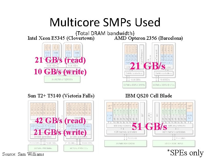
Multicore SMPs Used (Total DRAM bandwidth) Intel Xeon E 5345 (Clovertown) AMD Opteron 2356 (Barcelona) 21 GB/s (read) 10 GB/s (write) 21 GB/s Sun T 2+ T 5140 (Victoria Falls) IBM QS 20 Cell Blade 42 GB/s (read) 21 GB/s (write) 51 GB/s Source: Sam Williams *SPEs only

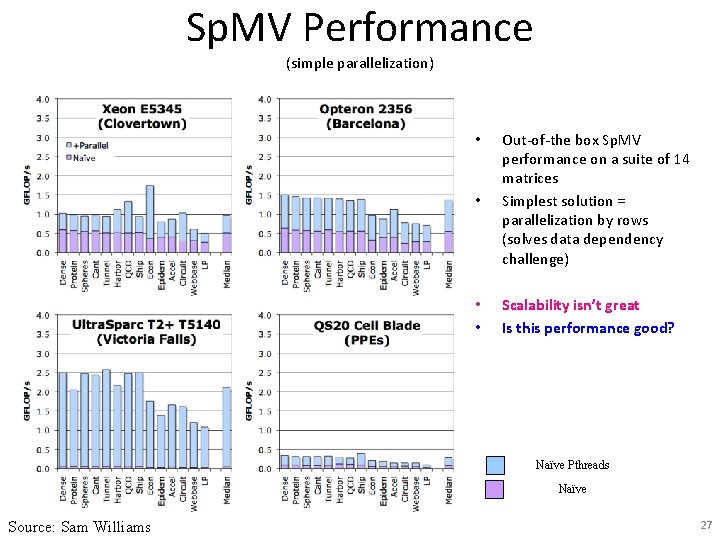
Sp. MV Performance (simple parallelization) • Out-of-the box Sp. MV performance on a suite of 14 matrices Simplest solution = parallelization by rows (solves data dependency challenge) • • Scalability isn’t great Is this performance good? • Naïve Pthreads Naïve Source: Sam Williams 27

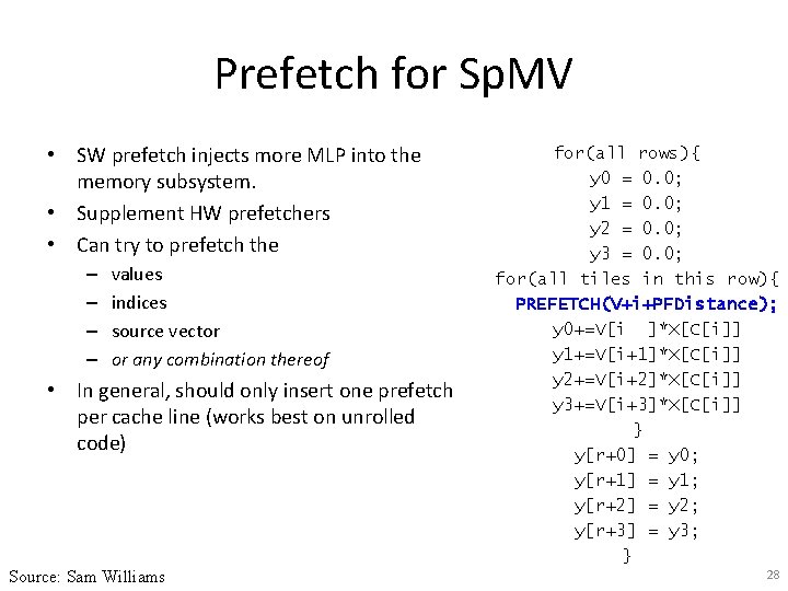
Prefetch for Sp. MV • SW prefetch injects more MLP into the memory subsystem. • Supplement HW prefetchers • Can try to prefetch the – – values indices source vector or any combination thereof • In general, should only insert one prefetch per cache line (works best on unrolled code) Source: Sam Williams for(all rows){ y 0 = 0. 0; y 1 = 0. 0; y 2 = 0. 0; y 3 = 0. 0; for(all tiles in this row){ PREFETCH(V+i+PFDistance); y 0+=V[i ]*X[C[i]] y 1+=V[i+1]*X[C[i]] y 2+=V[i+2]*X[C[i]] y 3+=V[i+3]*X[C[i]] } y[r+0] = y 0; y[r+1] = y 1; y[r+2] = y 2; y[r+3] = y 3; } 28

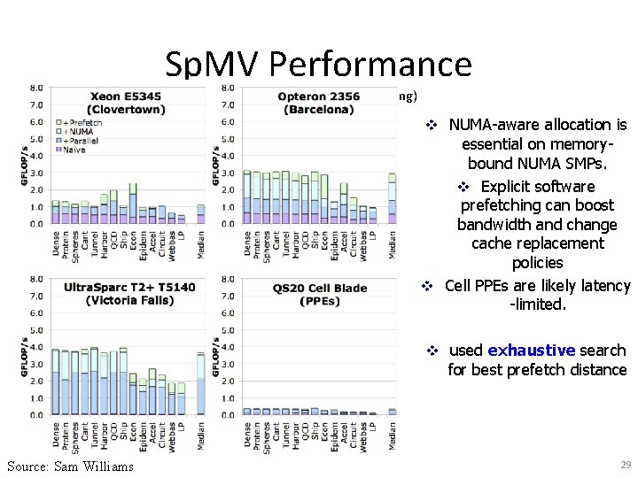
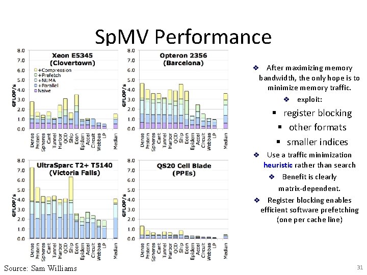
Sp. MV Performance (NUMA and Software Prefetching) v NUMA-aware allocation is essential on memorybound NUMA SMPs. v Explicit software prefetching can boost bandwidth and change cache replacement policies v Cell PPEs are likely latency -limited. v used exhaustive search for best prefetch distance Source: Sam Williams 29

Sp. MV Performance (Matrix Compression) After maximizing memory bandwidth, the only hope is to minimize memory traffic. v exploit: v § register blocking § other formats § smaller indices Use a traffic minimization heuristic rather than search v Benefit is clearly matrix-dependent. v Register blocking enables efficient software prefetching (one per cache line) v Source: Sam Williams 31

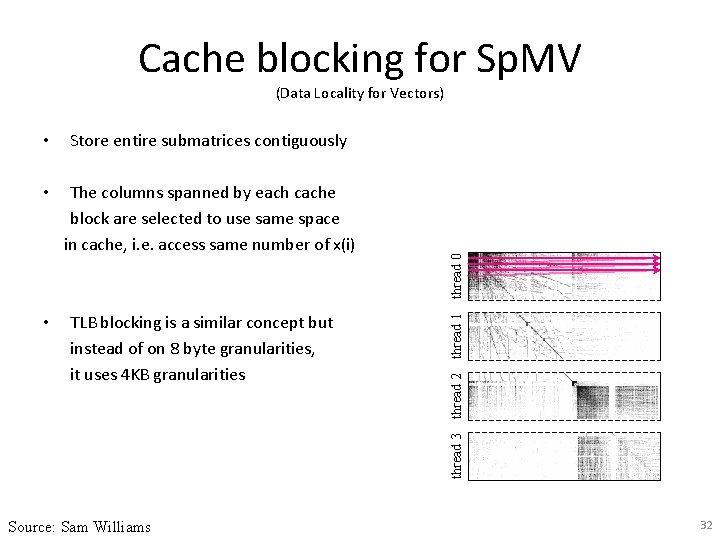
Cache blocking for Sp. MV • The columns spanned by each cache block are selected to use same space in cache, i. e. access same number of x(i) TLB blocking is a similar concept but instead of on 8 byte granularities, it uses 4 KB granularities thread 3 • thread 1 Store entire submatrices contiguously thread 2 • thread 0 (Data Locality for Vectors) Source: Sam Williams 32

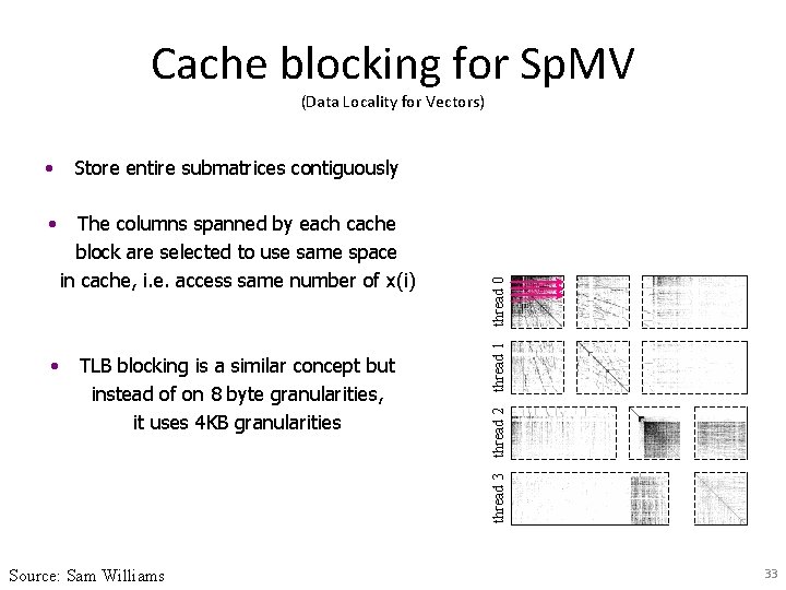
Cache blocking for Sp. MV The columns spanned by each cache block are selected to use same space in cache, i. e. access same number of x(i) • TLB blocking is a similar concept but instead of on 8 byte granularities, it uses 4 KB granularities thread 1 • thread 2 Store entire submatrices contiguously thread 3 • thread 0 (Data Locality for Vectors) Source: Sam Williams 33

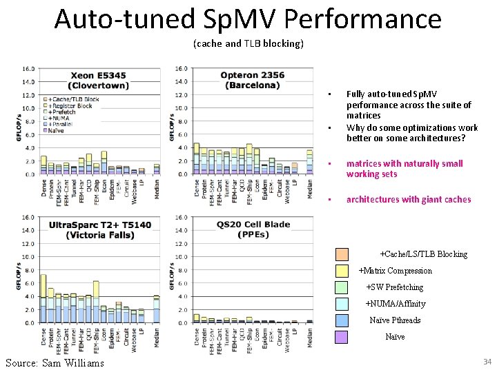
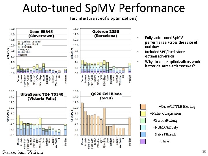
Auto-tuned Sp. MV Performance (cache and TLB blocking) • • Fully auto-tuned Sp. MV performance across the suite of matrices Why do some optimizations work better on some architectures? • matrices with naturally small working sets • architectures with giant caches +Cache/LS/TLB Blocking +Matrix Compression +SW Prefetching +NUMA/Affinity Naïve Pthreads Naïve Source: Sam Williams 34

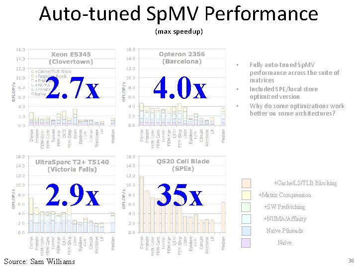
Auto-tuned Sp. MV Performance (architecture specific optimizations) • • • Fully auto-tuned Sp. MV performance across the suite of matrices Included SPE/local store optimized version Why do some optimizations work better on some architectures? +Cache/LS/TLB Blocking +Matrix Compression +SW Prefetching +NUMA/Affinity Naïve Pthreads Naïve Source: Sam Williams 35

Auto-tuned Sp. MV Performance (max speedup) • 2. 7 x 4. 0 x 2. 9 x 35 x • • Fully auto-tuned Sp. MV performance across the suite of matrices Included SPE/local store optimized version Why do some optimizations work better on some architectures? +Cache/LS/TLB Blocking +Matrix Compression +SW Prefetching +NUMA/Affinity Naïve Pthreads Naïve Source: Sam Williams 36

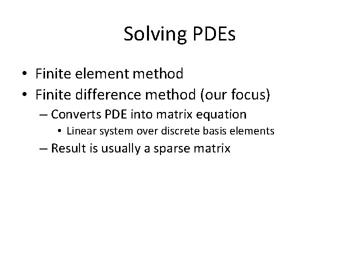
Solving PDEs • Finite element method • Finite difference method (our focus) – Converts PDE into matrix equation • Linear system over discrete basis elements – Result is usually a sparse matrix

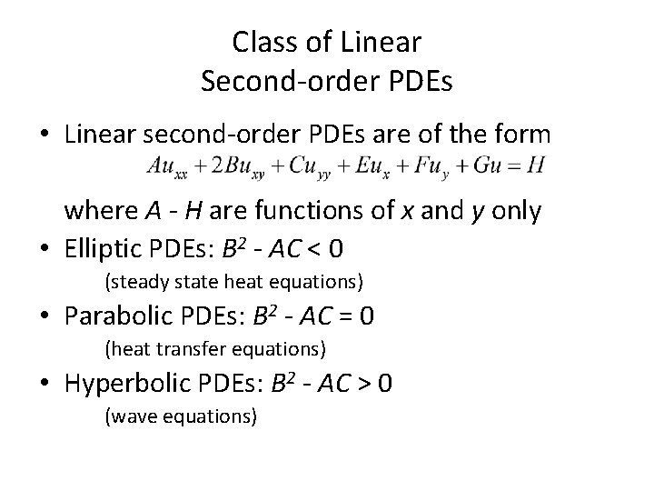
Class of Linear Second-order PDEs • Linear second-order PDEs are of the form where A - H are functions of x and y only • Elliptic PDEs: B 2 - AC < 0 (steady state heat equations) • Parabolic PDEs: B 2 - AC = 0 (heat transfer equations) • Hyperbolic PDEs: B 2 - AC > 0 (wave equations)

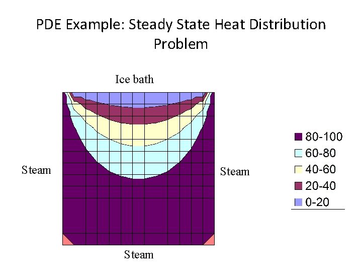
PDE Example: Steady State Heat Distribution Problem Ice bath Steam

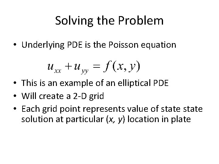
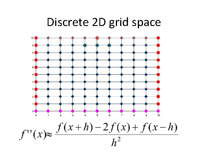
Solving the Problem • Underlying PDE is the Poisson equation • This is an example of an elliptical PDE • Will create a 2 -D grid • Each grid point represents value of state solution at particular (x, y) location in plate

Discrete 2 D grid space

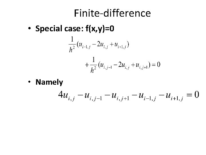
Finite-difference • Special case: f(x, y)=0 • Namely

Heart of Iterative Program w[i][j] = (u[i-1][j] + u[i+1][j] + u[i][j-1] + u[i][j+1]) / 4. 0;

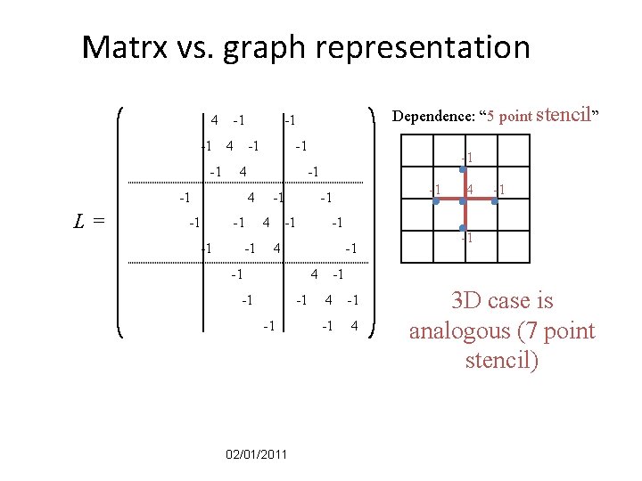
Matrx vs. graph representation 4 -1 -1 -1 4 -1 L= -1 4 -1 -1 -1 4 -1 Dependence: “ 5 point stencil” -1 -1 -1 4 -1 -1 -1 02/01/2011 4 -1 -1 -1 4 3 D case is analogous (7 point stencil)

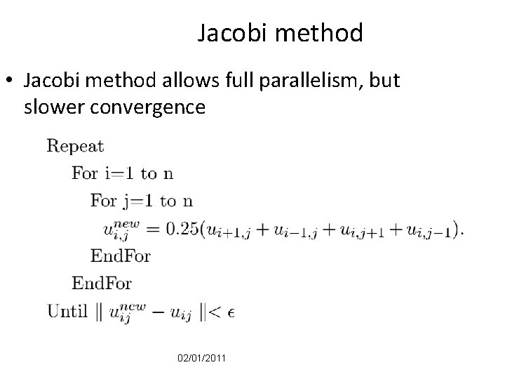
Jacobi method • Jacobi method allows full parallelism, but slower convergence 02/01/2011

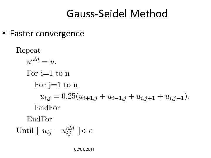
Gauss-Seidel Method • Faster convergence 02/01/2011

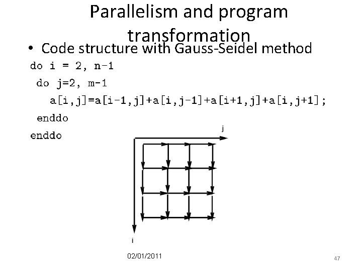
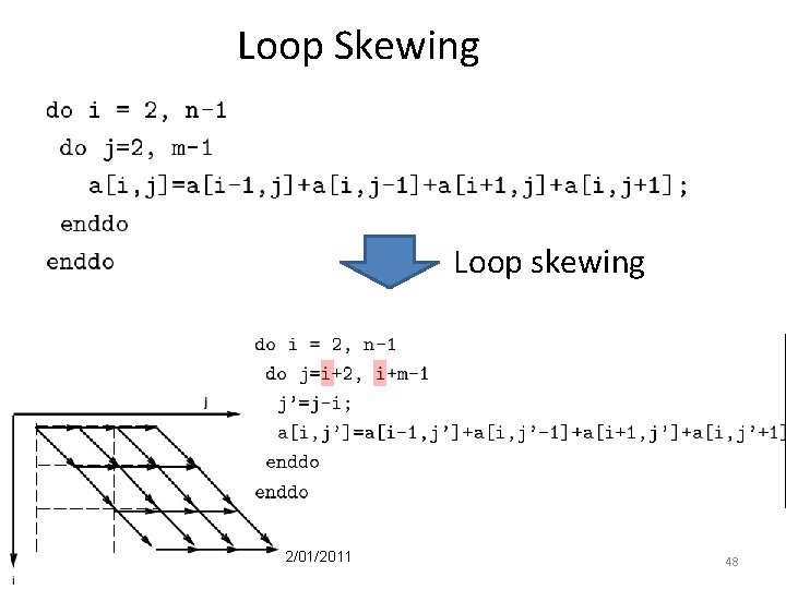
Parallelism and program transformation • Code structure with Gauss-Seidel method 02/01/2011 47

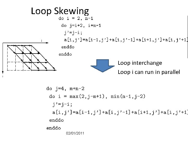
Loop Skewing Loop skewing 02/01/2011 48

Loop Skewing Loop interchange Loop i can run in parallel 02/01/2011

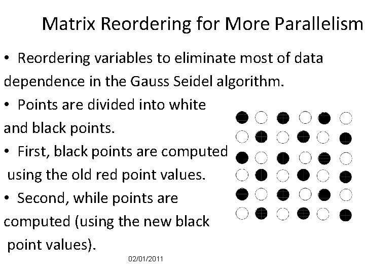
Matrix Reordering for More Parallelism • Reordering variables to eliminate most of data dependence in the Gauss Seidel algorithm. • Points are divided into white and black points. • First, black points are computed using the old red point values. • Second, while points are computed (using the new black point values). 02/01/2011

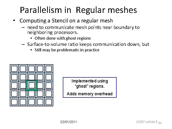
Parallelism in Regular meshes • Computing a Stencil on a regular mesh – need to communicate mesh points near boundary to neighboring processors. • Often done with ghost regions – Surface-to-volume ratio keeps communication down, but • Still may be problematic in practice Implemented using “ghost” regions. Adds memory overhead 02/01/2011 CS 267 Lecture 5 51

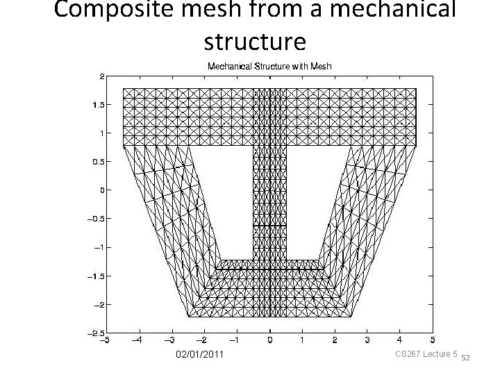
Composite mesh from a mechanical structure 02/01/2011 CS 267 Lecture 5 52

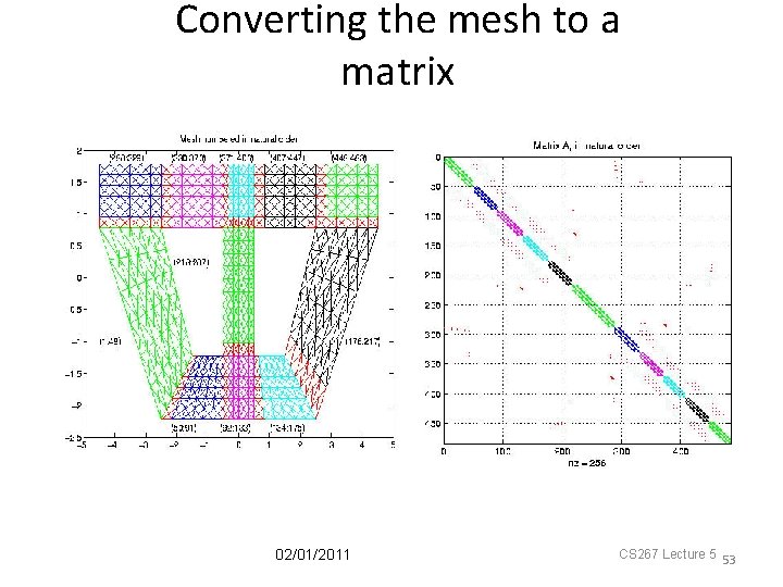
Converting the mesh to a matrix 02/01/2011 CS 267 Lecture 5 53

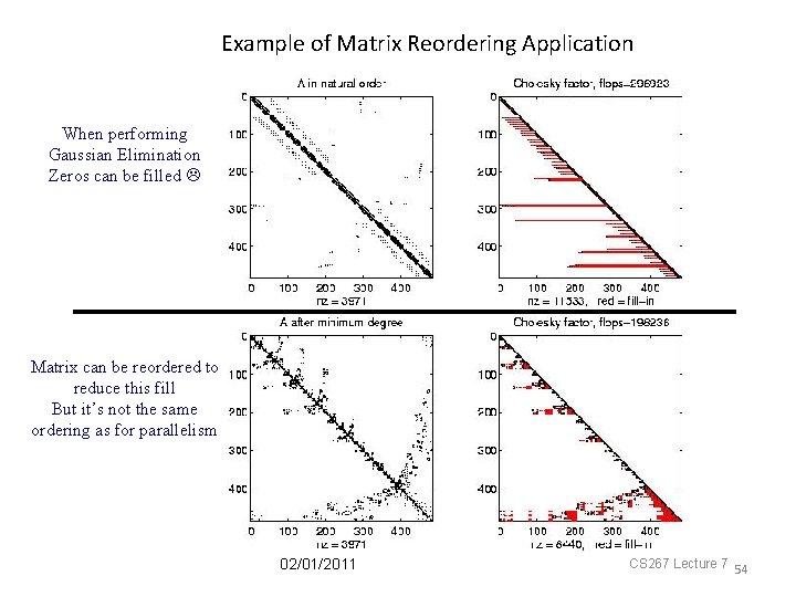
Example of Matrix Reordering Application When performing Gaussian Elimination Zeros can be filled Matrix can be reordered to reduce this fill But it’s not the same ordering as for parallelism 02/01/2011 CS 267 Lecture 7 54

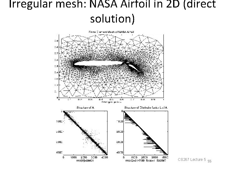
Irregular mesh: NASA Airfoil in 2 D (direct solution) 02/01/2011 CS 267 Lecture 5 55

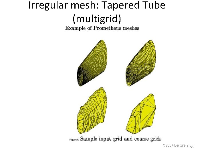
Irregular mesh: Tapered Tube (multigrid) 02/01/2011 CS 267 Lecture 9 56

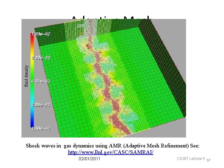
fluid density Adaptive Mesh Shock waves in gas dynamics using AMR (Adaptive Mesh Refinement) See: http: //www. llnl. gov/CASC/SAMRAI/ 02/01/2011 CS 267 Lecture 5 57

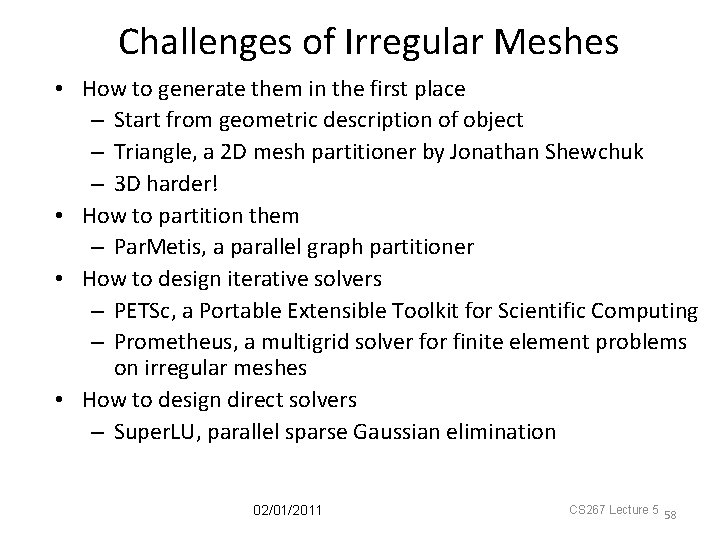
Challenges of Irregular Meshes • How to generate them in the first place – Start from geometric description of object – Triangle, a 2 D mesh partitioner by Jonathan Shewchuk – 3 D harder! • How to partition them – Par. Metis, a parallel graph partitioner • How to design iterative solvers – PETSc, a Portable Extensible Toolkit for Scientific Computing – Prometheus, a multigrid solver for finite element problems on irregular meshes • How to design direct solvers – Super. LU, parallel sparse Gaussian elimination 02/01/2011 CS 267 Lecture 5 58