PART 7 Ordinary Differential Equations ODEs Ordinary Differential

PART 7 Ordinary Differential Equations ODEs

Ordinary Differential Equations Part 7 • Equations which are composed of an unknown function and its derivatives are called differential equations. v - dependent variable t - independent variable • Differential equations play a fundamental role in engineering because many physical phenomena are best formulated mathematically in terms of their rate of change.

Ordinary Differential Equations • When a function involves one dependent variable, the equation is called an ordinary differential equation (ODE). • A partial differential equation (PDE) involves two or more independent variables.

Ordinary Differential Equations Differential equations are also classified as to their order: 1. A first order equation includes a first derivative as its highest derivative. - Linear 1 st order ODE - Non-Linear 1 st order ODE Where f(x, y) is nonlinear

Ordinary Differential Equations 2. A second order equation includes a second derivative. - Linear 2 nd order ODE - Non-Linear 2 nd order ODE • Higher order equations can be reduced to a system of first order equations, by redefining a variable.

Ordinary Differential Equations

Runge-Kutta Methods This chapter is devoted to solving ODE of the form: • Euler’s Method solution

Runge-Kutta Methods

Euler’s Method: Example Obtain a solution between x = 0 to x = 4 with a step size of 0. 5 for: Initial conditions are: x = 0 to y = 1 Solution:

Euler’s Method: Example • Although the computation captures the general trend solution, the error is considerable. • This error can be reduced by using a smaller step size.

Improvements of Euler’s method • A fundamental source of error in Euler’s method is that the derivative at the beginning of the interval is assumed to apply across the entire interval. • Simple modifications are available: – Heun’s Method – The Midpoint Method – Ralston’s Method

Runge-Kutta Methods • Runge-Kutta methods achieve the accuracy of a Taylor series approach without requiring the calculation of higher derivatives. Increment function (representative slope over the interval)

Runge-Kutta Methods Various types of RK methods can be devised by employing different number of terms in the increment function as specified by n. 1. First order RK method with n=1 is Euler’s method. • – Error is proportional to O(h) 2. Second order RK methods: - Error is proportional to O(h 2) • Values of a 1, a 2, p 1, and q 11 are evaluated by setting the second order equation to Taylor series expansion to the second order term.

Runge-Kutta Methods • Three equations to evaluate the four unknown constants are derived: A value is assumed for one of the unknowns to solve for the other three.

Runge-Kutta Methods • We can choose an infinite number of values for a 2, there an infinite number of second-order RK methods. • Every version would yield exactly the same results if the solution to ODE were quadratic, linear, or a constant. • However, they yield different results if the solution is more complicated (typically the case).

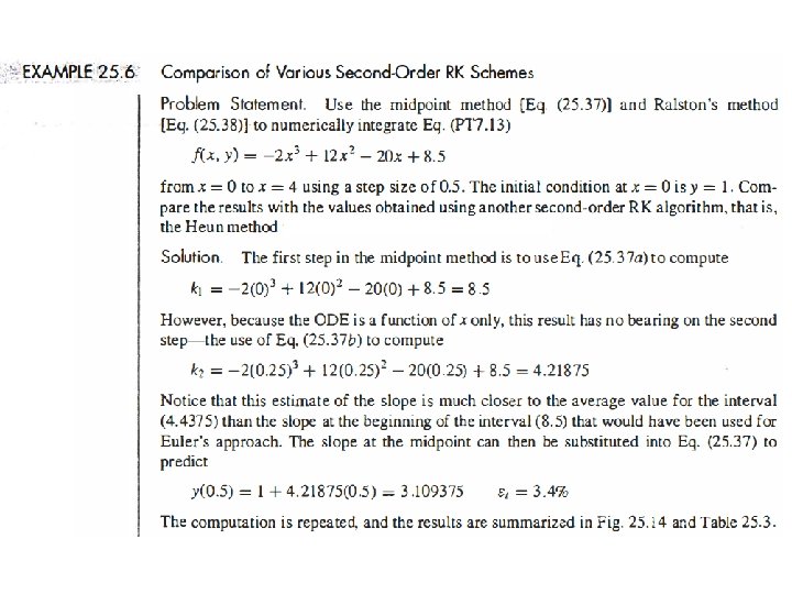
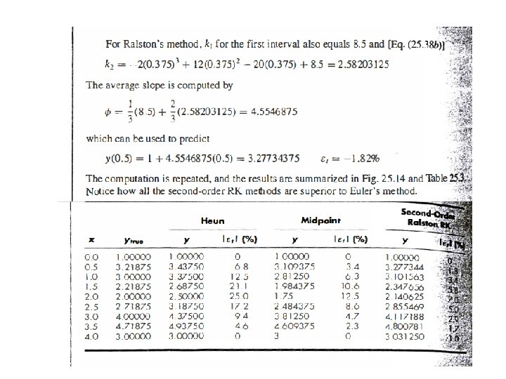
Runge-Kutta Methods Three of the most commonly used methods are: • Huen Method with a Single Corrector (a 2=1/2) • The Midpoint Method (a 2= 1) • Raltson’s Method (a 2= 2/3)

Runge-Kutta Methods y • Heun’s Method: Involves the determination of two derivatives for the interval at the initial point and the end point. f(xi, yi) xi f(xi+h, yi+k 1 h) x xi+h y ea Slope: 0. 5(k 1+k 2) xi xi+h x

Runge-Kutta Methods y • Midpoint Method: Uses Euler’s method to predict a value of y at the midpoint of the interval: f(xi, yi) xi f(xi+h/2, yi+k 1 h/2) x xi+h/2 y ea Slope: k 2 Chapter 25 xi xi+h x

Runge-Kutta Methods y • Ralston’s Method: f(xi, yi) xi f(xi+ 3/4 h, yi+3/4 k 1 h) xi+3/4 h x y ea Slope: (1/3 k 1+2/3 k 2) Chapter 25 xi xi+h x

Chapter 25 22

Runge-Kutta Methods 3. Third order RK methods Chapter 25

Runge-Kutta Methods 4. Fourth order RK methods Chapter 25

Comparison of Runge-Kutta Methods Use first to fourth order RK methods to solve the equation from x = 0 to x = 4 Initial condition y(0) = 2, exact answer of y(4) = 75. 33896 Chapter 25