Ch 6 4 Differential Equations with Discontinuous Forcing

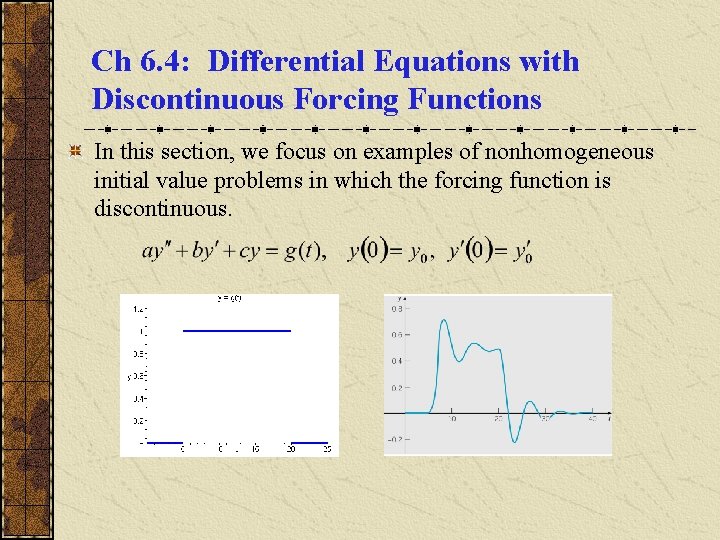
Ch 6. 4: Differential Equations with Discontinuous Forcing Functions In this section, we focus on examples of nonhomogeneous initial value problems in which the forcing function is discontinuous.

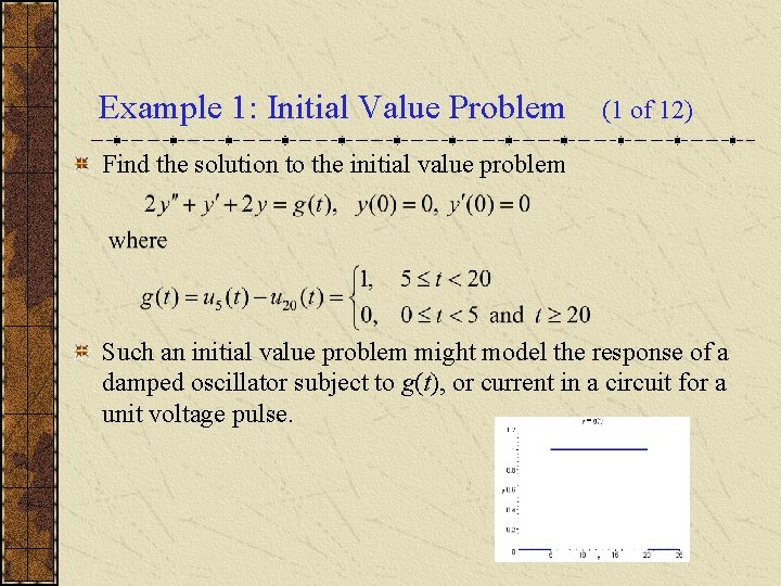
Example 1: Initial Value Problem (1 of 12) Find the solution to the initial value problem Such an initial value problem might model the response of a damped oscillator subject to g(t), or current in a circuit for a unit voltage pulse.

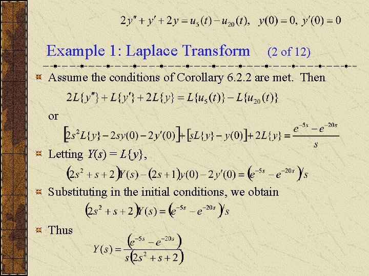
Example 1: Laplace Transform (2 of 12) Assume the conditions of Corollary 6. 2. 2 are met. Then or Letting Y(s) = L{y}, Substituting in the initial conditions, we obtain Thus

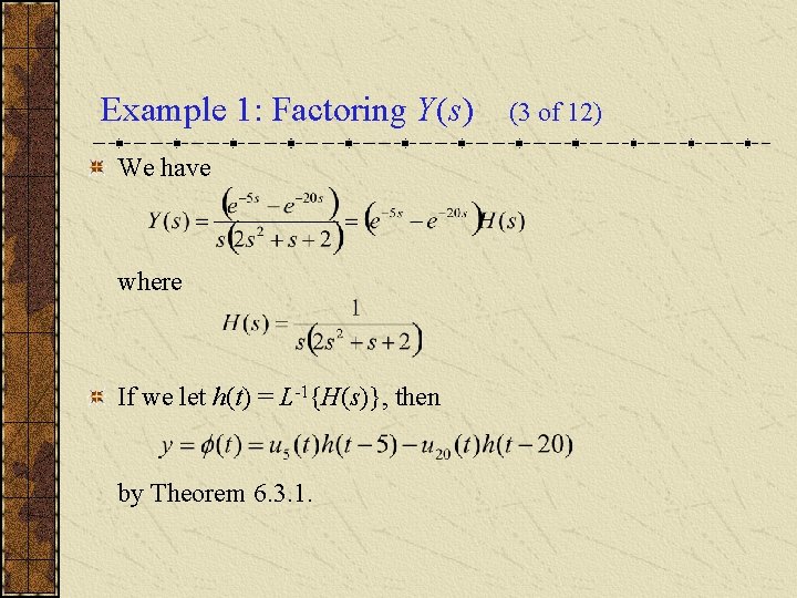
Example 1: Factoring Y(s) We have where If we let h(t) = L-1{H(s)}, then by Theorem 6. 3. 1. (3 of 12)

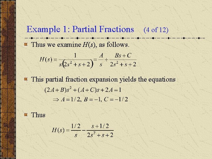
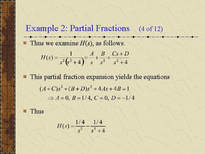
Example 1: Partial Fractions (4 of 12) Thus we examine H(s), as follows. This partial fraction expansion yields the equations Thus

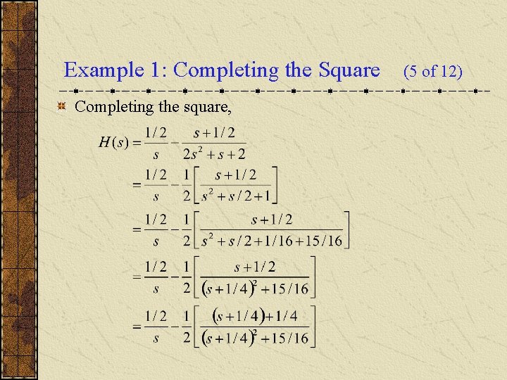
Example 1: Completing the Square Completing the square, (5 of 12)

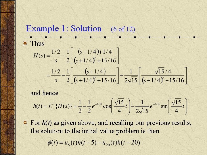
Example 1: Solution (6 of 12) Thus and hence For h(t) as given above, and recalling our previous results, the solution to the initial value problem is then

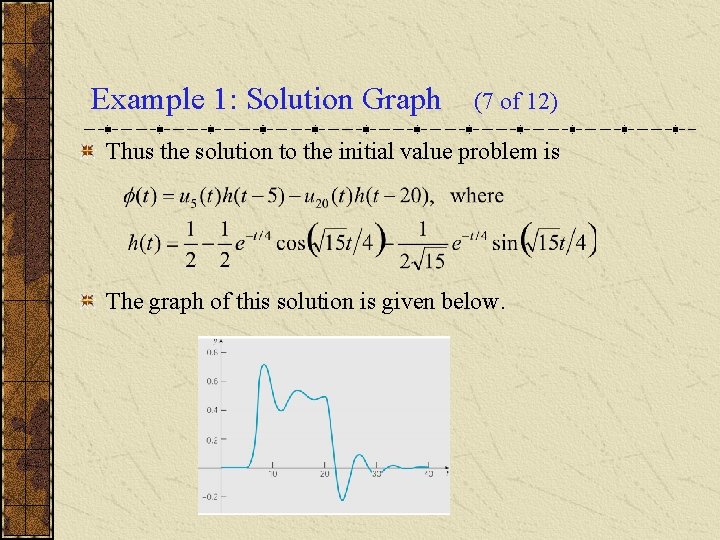
Example 1: Solution Graph (7 of 12) Thus the solution to the initial value problem is The graph of this solution is given below.

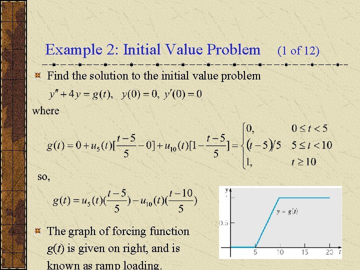
Example 2: Initial Value Problem Find the solution to the initial value problem The graph of forcing function g(t) is given on right, and is known as ramp loading. (1 of 12)

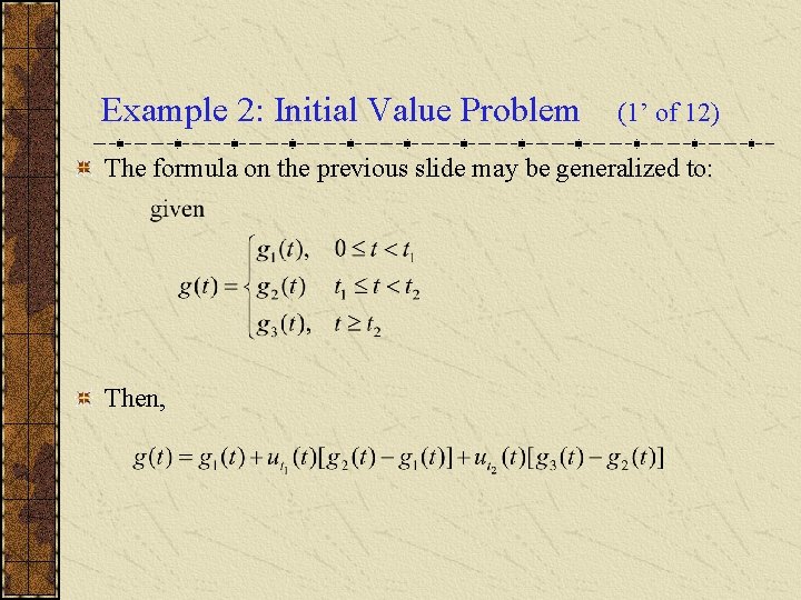
Example 2: Initial Value Problem (1’ of 12) The formula on the previous slide may be generalized to: Then,

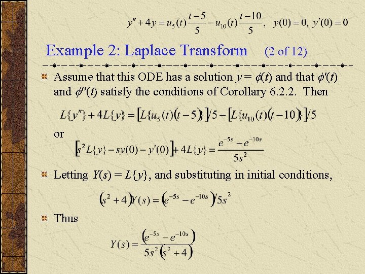
Example 2: Laplace Transform (2 of 12) Assume that this ODE has a solution y = (t) and that '(t) and ''(t) satisfy the conditions of Corollary 6. 2. 2. Then or Letting Y(s) = L{y}, and substituting in initial conditions, Thus

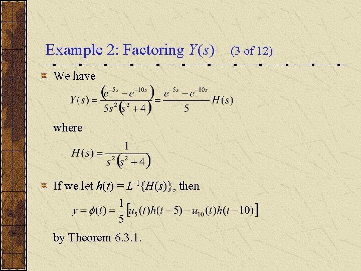
Example 2: Factoring Y(s) We have where If we let h(t) = L-1{H(s)}, then by Theorem 6. 3. 1. (3 of 12)

Example 2: Partial Fractions (4 of 12) Thus we examine H(s), as follows. This partial fraction expansion yields the equations Thus

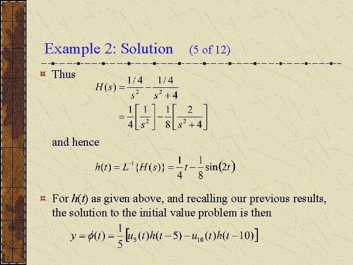
Example 2: Solution (5 of 12) Thus and hence For h(t) as given above, and recalling our previous results, the solution to the initial value problem is then

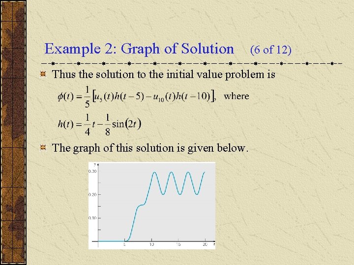
Example 2: Graph of Solution (6 of 12) Thus the solution to the initial value problem is The graph of this solution is given below.