9 DIFFERENTIAL EQUATIONS DIFFERENTIAL EQUATIONS 9 4 Models

9 DIFFERENTIAL EQUATIONS

DIFFERENTIAL EQUATIONS 9. 4 Models for Population Growth In this section, we will: Investigate differential equations used to model population growth.

NATURAL GROWTH One of the models for population growth we considered in Section 9. 1 was based on the assumption that the population grows at a rate proportional to the size of the population:

NATURAL GROWTH Is that a reasonable assumption?

NATURAL GROWTH Suppose we have a population (of bacteria, for instance) with size P = 1000. § At a certain time, it is growing at a rate of P’ = 300 bacteria per hour.

NATURAL GROWTH Now, let’s take another 1, 000 bacteria of the same type and put them with the first population. § Each half of the new population was growing at a rate of 300 bacteria per hour.

NATURAL GROWTH We would expect the total population of 2, 000 to increase at a rate of 600 bacteria per hour initially—provided there’s enough room and nutrition. § So, if we double the size, we double the growth rate.

NATURAL GROWTH In general, it seems reasonable that the growth rate should be proportional to the size.

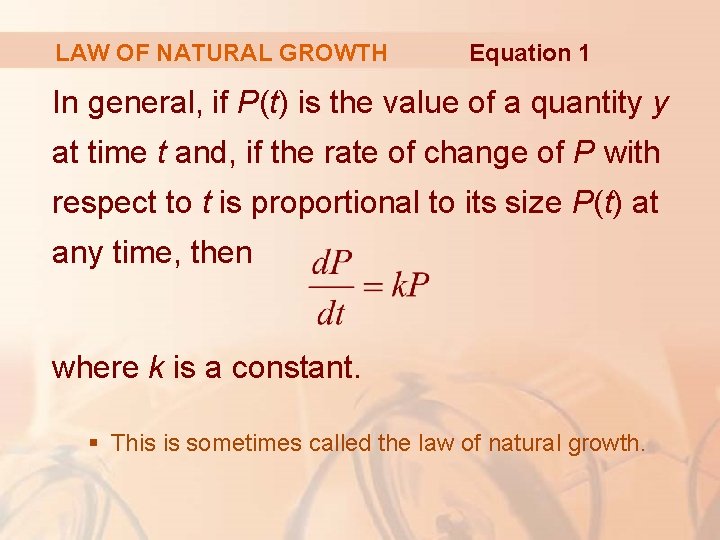
LAW OF NATURAL GROWTH Equation 1 In general, if P(t) is the value of a quantity y at time t and, if the rate of change of P with respect to t is proportional to its size P(t) at any time, then where k is a constant. § This is sometimes called the law of natural growth.

LAW OF NATURAL GROWTH If k is positive, the population increases. If k is negative, it decreases.

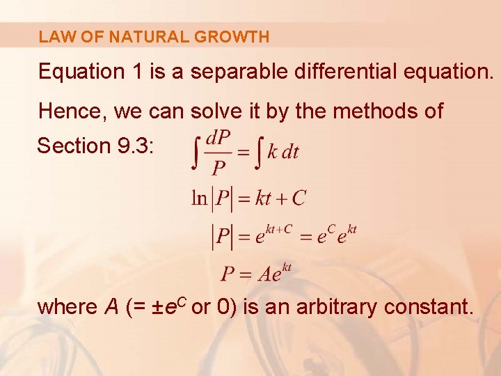
LAW OF NATURAL GROWTH Equation 1 is a separable differential equation. Hence, we can solve it by the methods of Section 9. 3: where A (= ±e. C or 0) is an arbitrary constant.

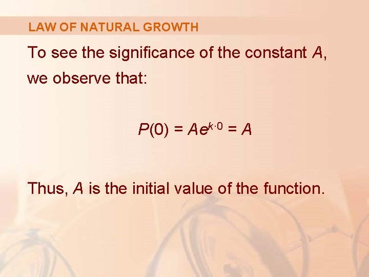
LAW OF NATURAL GROWTH To see the significance of the constant A, we observe that: P(0) = Aek· 0 = A Thus, A is the initial value of the function.

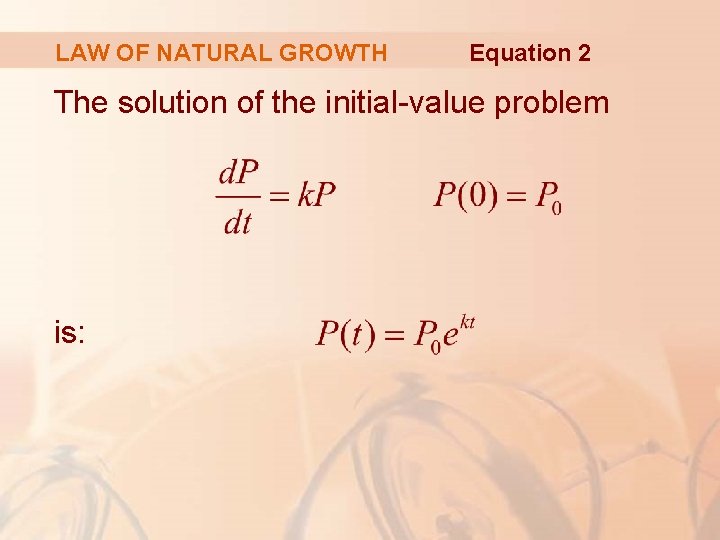
LAW OF NATURAL GROWTH Equation 2 The solution of the initial-value problem is:

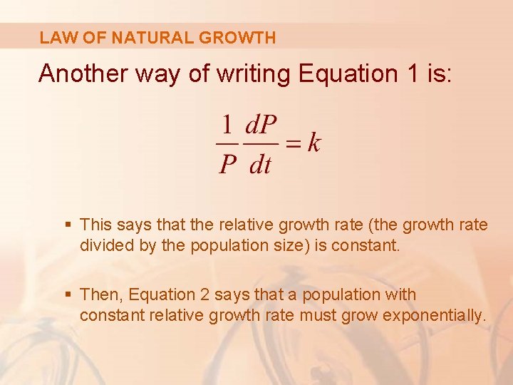
LAW OF NATURAL GROWTH Another way of writing Equation 1 is: § This says that the relative growth rate (the growth rate divided by the population size) is constant. § Then, Equation 2 says that a population with constant relative growth rate must grow exponentially.

LAW OF NATURAL GROWTH We can account for emigration (or “harvesting”) from a population by modifying Equation 1—as follows.

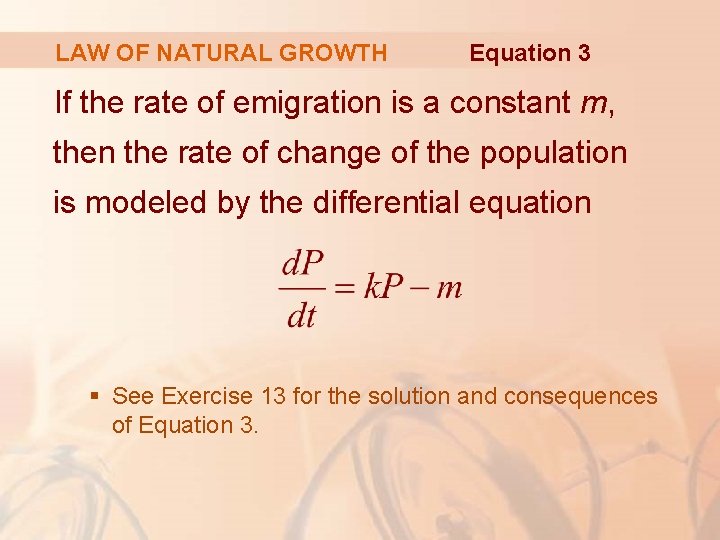
LAW OF NATURAL GROWTH Equation 3 If the rate of emigration is a constant m, then the rate of change of the population is modeled by the differential equation § See Exercise 13 for the solution and consequences of Equation 3.

LOGISTIC MODEL As we discussed in Section 9. 1, a population often increases exponentially in its early stages, but levels off eventually and approaches its carrying capacity because of limited resources.

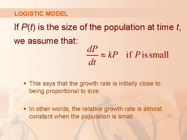
LOGISTIC MODEL If P(t) is the size of the population at time t, we assume that: § This says that the growth rate is initially close to being proportional to size. § In other words, the relative growth rate is almost constant when the population is small.

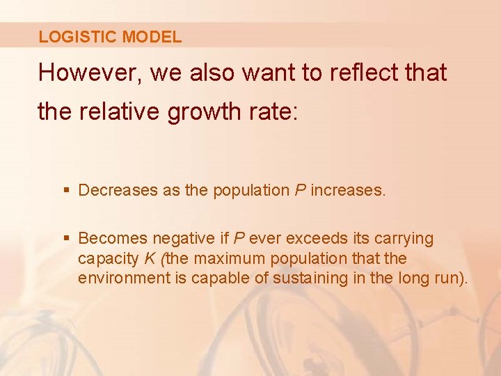
LOGISTIC MODEL However, we also want to reflect that the relative growth rate: § Decreases as the population P increases. § Becomes negative if P ever exceeds its carrying capacity K (the maximum population that the environment is capable of sustaining in the long run).

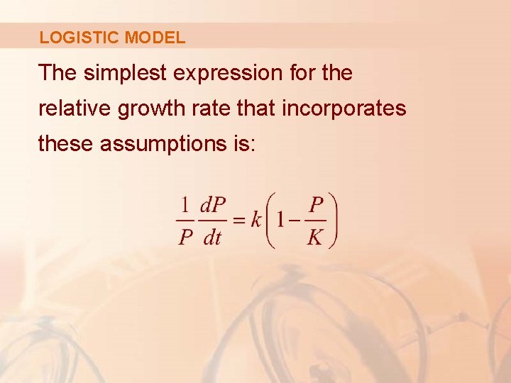
LOGISTIC MODEL The simplest expression for the relative growth rate that incorporates these assumptions is:

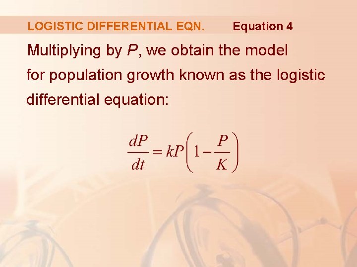
LOGISTIC DIFFERENTIAL EQN. Equation 4 Multiplying by P, we obtain the model for population growth known as the logistic differential equation:

LOGISTIC DIFFERENTIAL EQN. Notice from Equation 4 that: § If P is small compared with K, then P/K is close to 0, and so d. P/dt ≈ k. P. § If P → K (the population approaches its carrying capacity), then P/K → 1, so d. P/dt → 0.

LOGISTIC DIFFERENTIAL EQN. From Equation 4, we can deduce information about whether solutions increase or decrease directly.

LOGISTIC DIFFERENTIAL EQN. If the population P lies between 0 and K, the right side of the equation is positive. § So, d. P/dt > 0 and the population increases. If the population exceeds the carrying capacity (P > K), 1 – P/K is negative. § So, d. P/dt < 0 and the population decreases.

LOGISTIC DIFFERENTIAL EQN. Let’s start our more detailed analysis of the logistic differential equation by looking at a direction field.

LOGISTIC DIFFERENTIAL EQN. Example 1 Draw a direction field for the logistic equation with k = 0. 08 and carrying capacity K = 1000. What can you deduce about the solutions?

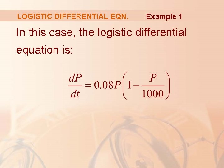
LOGISTIC DIFFERENTIAL EQN. Example 1 In this case, the logistic differential equation is:

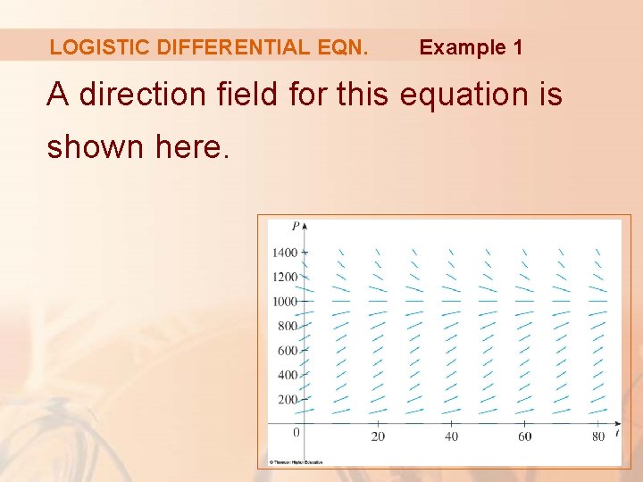
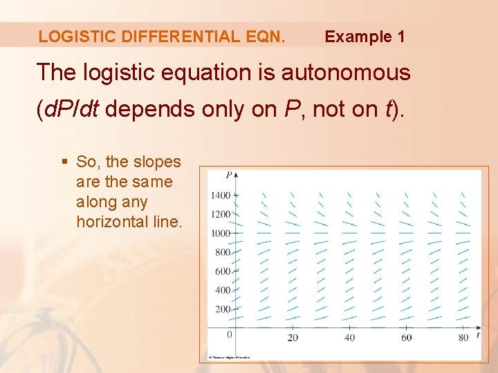
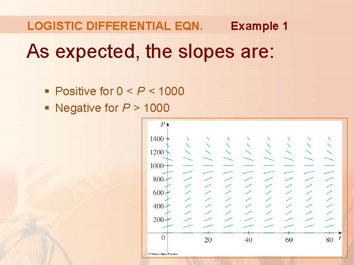
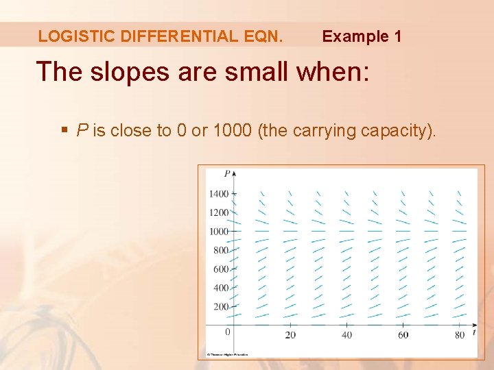
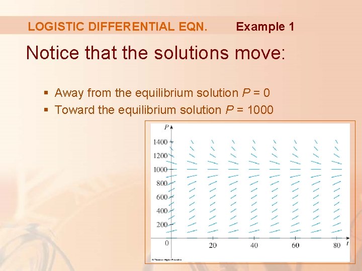
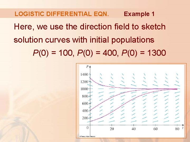
LOGISTIC DIFFERENTIAL EQN. Example 1 A direction field for this equation is shown here.

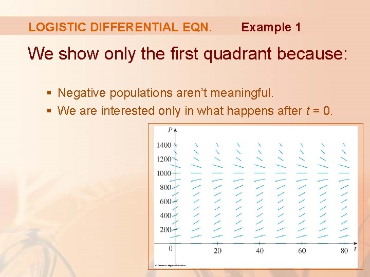
LOGISTIC DIFFERENTIAL EQN. Example 1 We show only the first quadrant because: § Negative populations aren’t meaningful. § We are interested only in what happens after t = 0.

LOGISTIC DIFFERENTIAL EQN. Example 1 The logistic equation is autonomous (d. P/dt depends only on P, not on t). § So, the slopes are the same along any horizontal line.

LOGISTIC DIFFERENTIAL EQN. Example 1 As expected, the slopes are: § Positive for 0 < P < 1000 § Negative for P > 1000

LOGISTIC DIFFERENTIAL EQN. Example 1 The slopes are small when: § P is close to 0 or 1000 (the carrying capacity).

LOGISTIC DIFFERENTIAL EQN. Example 1 Notice that the solutions move: § Away from the equilibrium solution P = 0 § Toward the equilibrium solution P = 1000

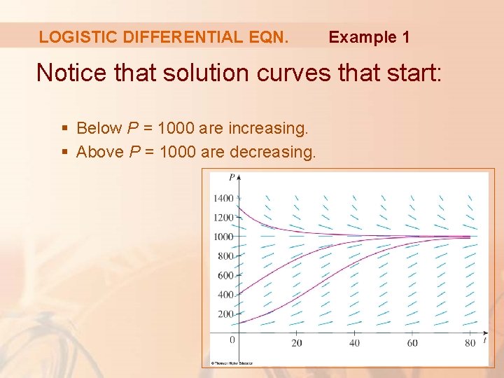
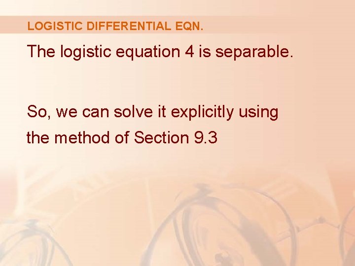
LOGISTIC DIFFERENTIAL EQN. Example 1 Here, we use the direction field to sketch solution curves with initial populations P(0) = 100, P(0) = 400, P(0) = 1300

LOGISTIC DIFFERENTIAL EQN. Example 1 Notice that solution curves that start: § Below P = 1000 are increasing. § Above P = 1000 are decreasing.

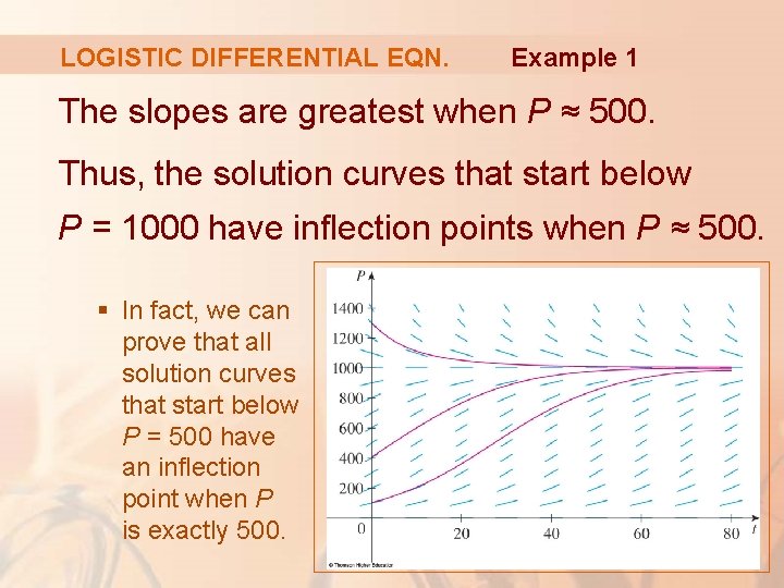
LOGISTIC DIFFERENTIAL EQN. Example 1 The slopes are greatest when P ≈ 500. Thus, the solution curves that start below P = 1000 have inflection points when P ≈ 500. § In fact, we can prove that all solution curves that start below P = 500 have an inflection point when P is exactly 500.

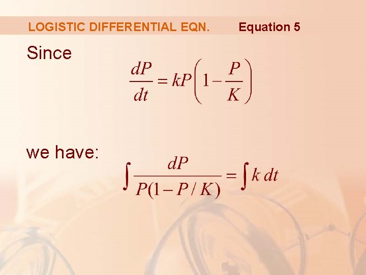
LOGISTIC DIFFERENTIAL EQN. The logistic equation 4 is separable. So, we can solve it explicitly using the method of Section 9. 3

LOGISTIC DIFFERENTIAL EQN. Since we have: Equation 5

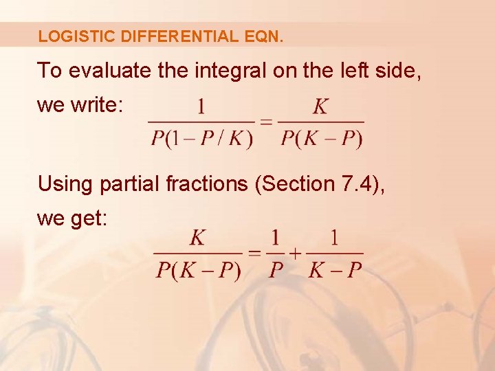
LOGISTIC DIFFERENTIAL EQN. To evaluate the integral on the left side, we write: Using partial fractions (Section 7. 4), we get:

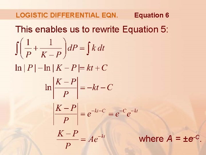
LOGISTIC DIFFERENTIAL EQN. Equation 6 This enables us to rewrite Equation 5: where A = ±e-C.

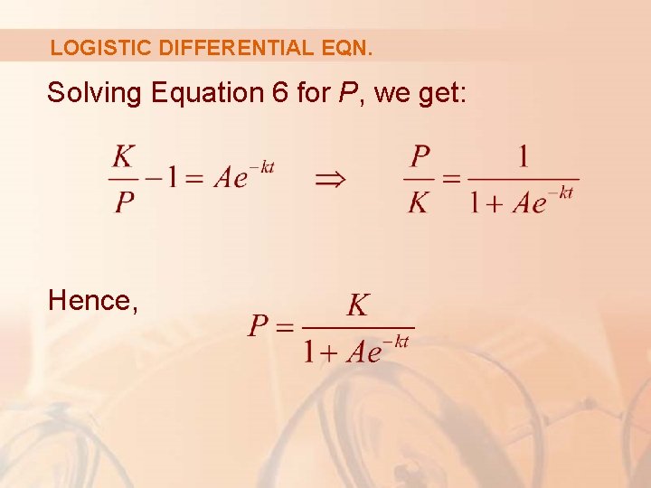
LOGISTIC DIFFERENTIAL EQN. Solving Equation 6 for P, we get: Hence,

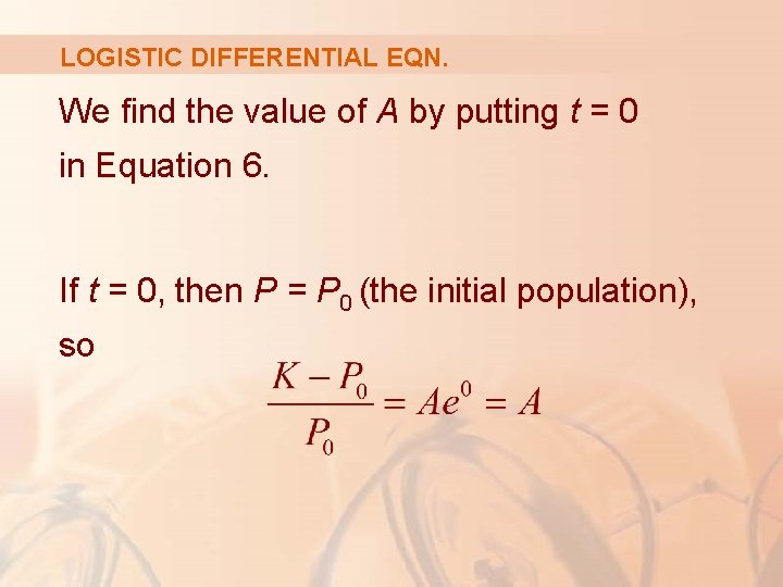
LOGISTIC DIFFERENTIAL EQN. We find the value of A by putting t = 0 in Equation 6. If t = 0, then P = P 0 (the initial population), so

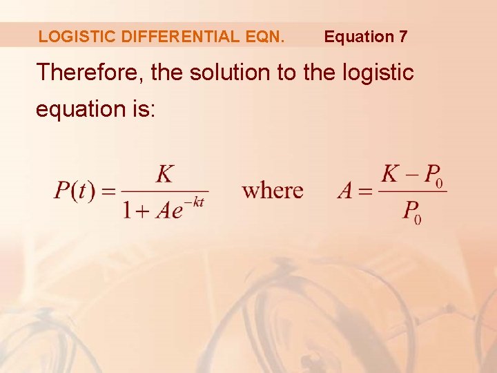
LOGISTIC DIFFERENTIAL EQN. Equation 7 Therefore, the solution to the logistic equation is:

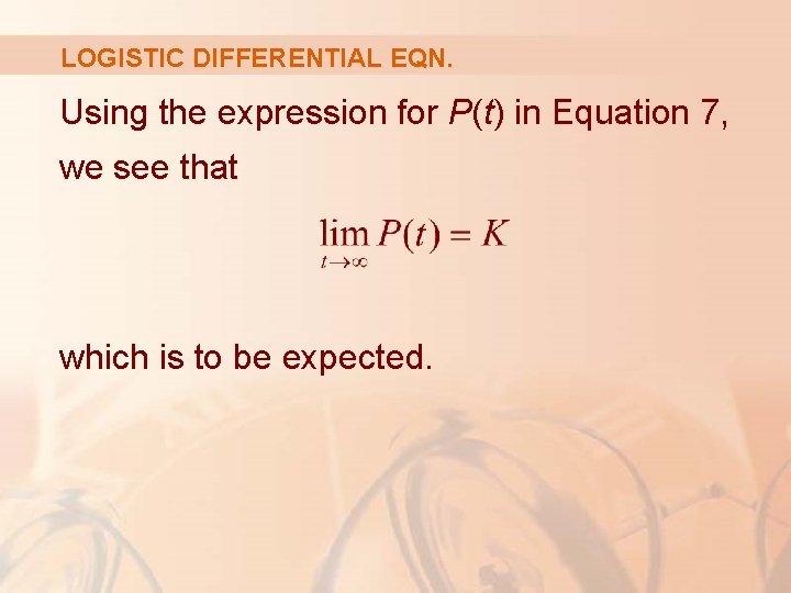
LOGISTIC DIFFERENTIAL EQN. Using the expression for P(t) in Equation 7, we see that which is to be expected.

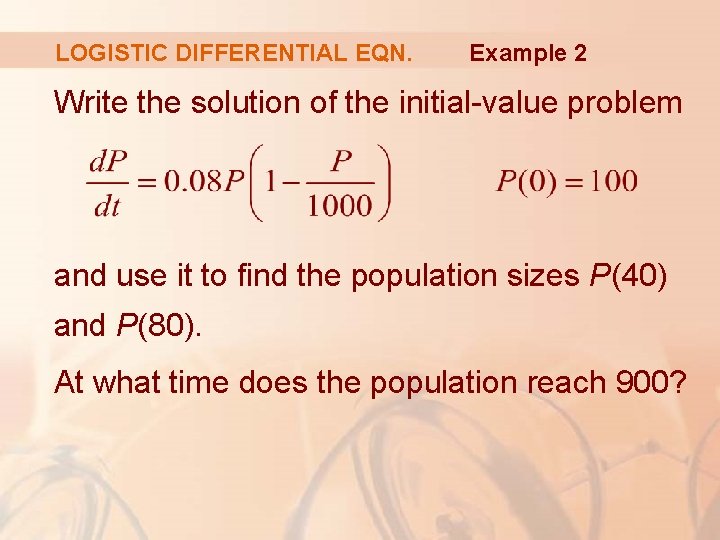
LOGISTIC DIFFERENTIAL EQN. Example 2 Write the solution of the initial-value problem and use it to find the population sizes P(40) and P(80). At what time does the population reach 900?

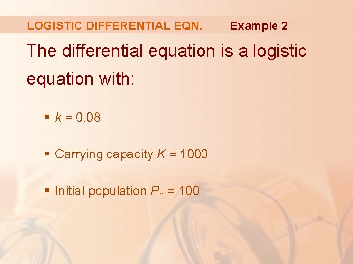
LOGISTIC DIFFERENTIAL EQN. Example 2 The differential equation is a logistic equation with: § k = 0. 08 § Carrying capacity K = 1000 § Initial population P 0 = 100

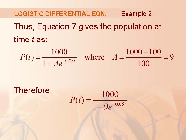
LOGISTIC DIFFERENTIAL EQN. Example 2 Thus, Equation 7 gives the population at time t as: Therefore,

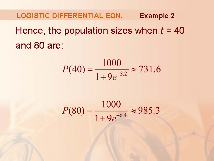
LOGISTIC DIFFERENTIAL EQN. Example 2 Hence, the population sizes when t = 40 and 80 are:

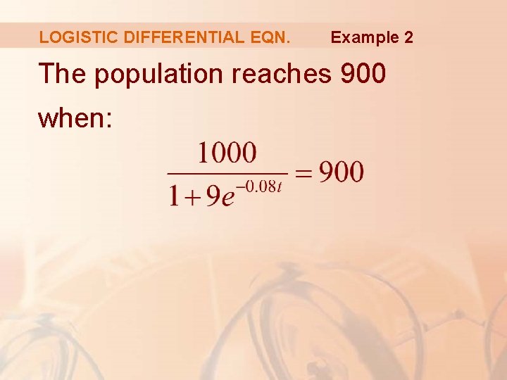
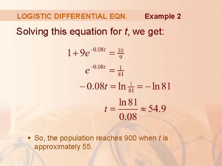
LOGISTIC DIFFERENTIAL EQN. Example 2 The population reaches 900 when:

LOGISTIC DIFFERENTIAL EQN. Example 2 Solving this equation for t, we get: § So, the population reaches 900 when t is approximately 55.

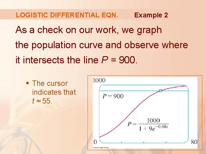
LOGISTIC DIFFERENTIAL EQN. Example 2 As a check on our work, we graph the population curve and observe where it intersects the line P = 900. § The cursor indicates that t ≈ 55.

COMPARING THE MODELS In the 1930 s, the biologist G. F. Gause conducted an experiment with the protozoan Paramecium and used a logistic equation to model his data.

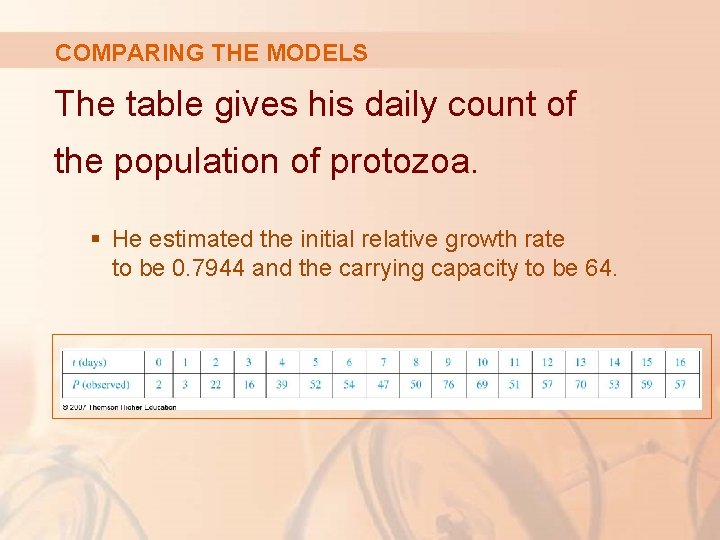
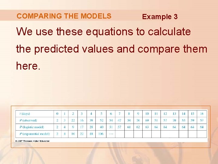
COMPARING THE MODELS The table gives his daily count of the population of protozoa. § He estimated the initial relative growth rate to be 0. 7944 and the carrying capacity to be 64.

COMPARING THE MODELS Example 3 Find the exponential and logistic models for Gause’s data. Compare the predicted values with the observed values and comment on the fit.

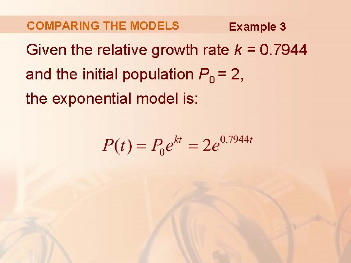
COMPARING THE MODELS Example 3 Given the relative growth rate k = 0. 7944 and the initial population P 0 = 2, the exponential model is:

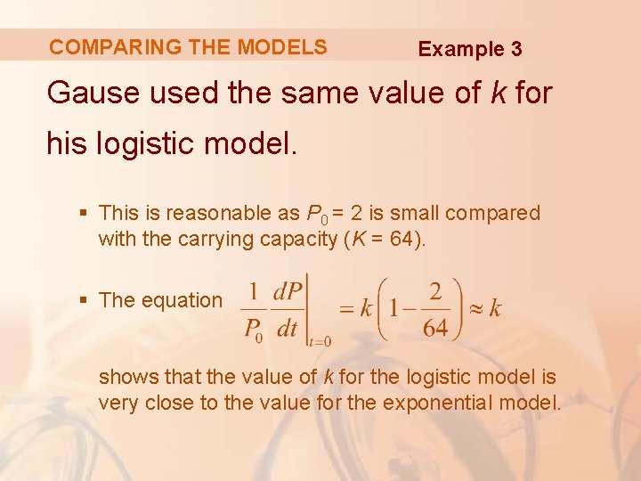
COMPARING THE MODELS Example 3 Gause used the same value of k for his logistic model. § This is reasonable as P 0 = 2 is small compared with the carrying capacity (K = 64). § The equation shows that the value of k for the logistic model is very close to the value for the exponential model.

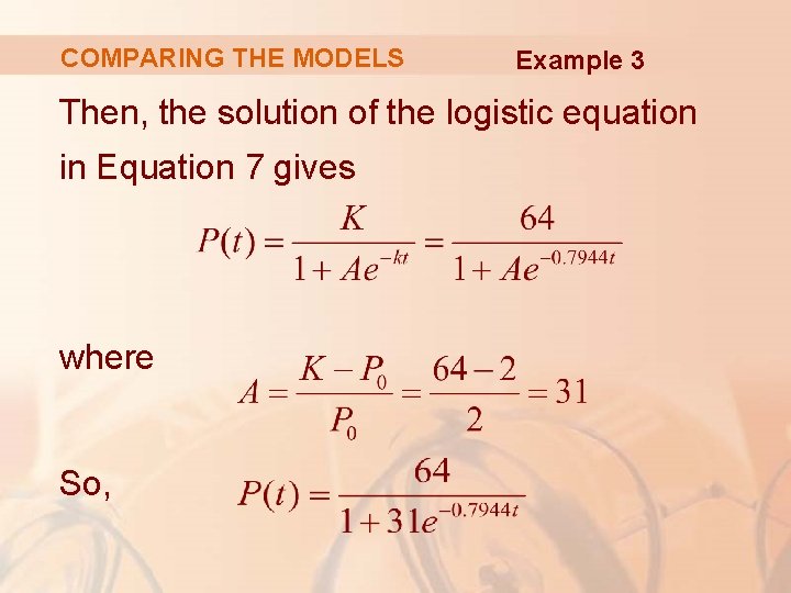
COMPARING THE MODELS Example 3 Then, the solution of the logistic equation in Equation 7 gives where So,

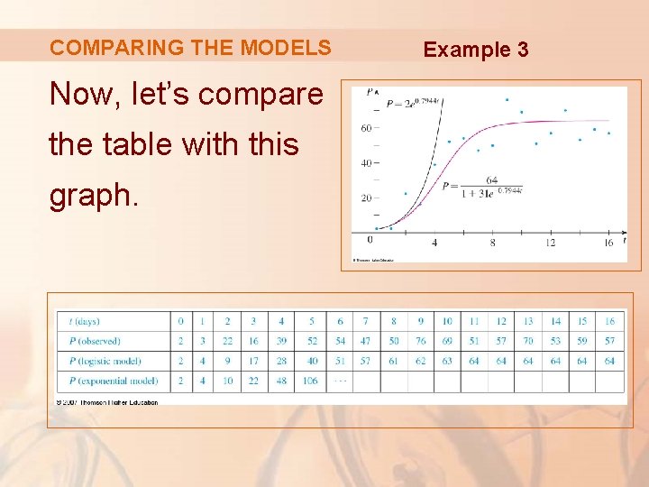
COMPARING THE MODELS Example 3 We use these equations to calculate the predicted values and compare them here.

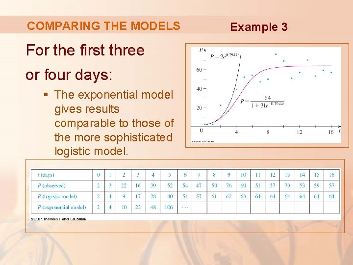
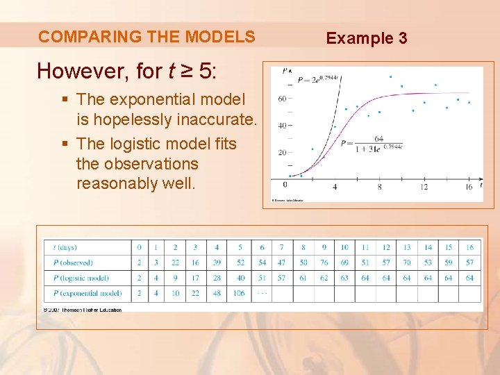
COMPARING THE MODELS Now, let’s compare the table with this graph. Example 3

COMPARING THE MODELS For the first three or four days: § The exponential model gives results comparable to those of the more sophisticated logistic model. Example 3

COMPARING THE MODELS However, for t ≥ 5: § The exponential model is hopelessly inaccurate. § The logistic model fits the observations reasonably well. Example 3

COMPARING THE MODELS Many countries that formerly experienced exponential growth are now finding that their rates of population growth are declining and the logistic model provides a better model.

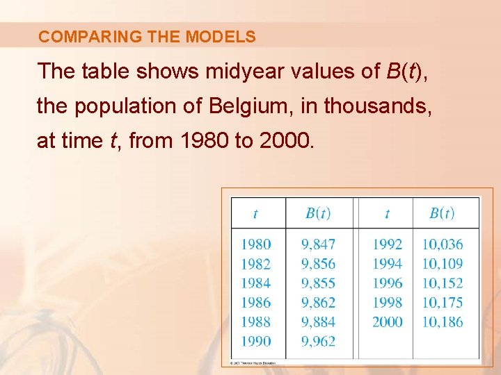
COMPARING THE MODELS The table shows midyear values of B(t), the population of Belgium, in thousands, at time t, from 1980 to 2000.

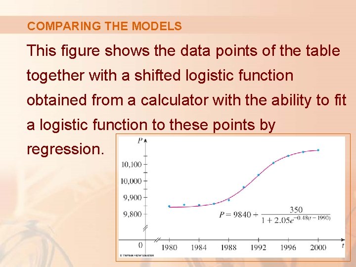
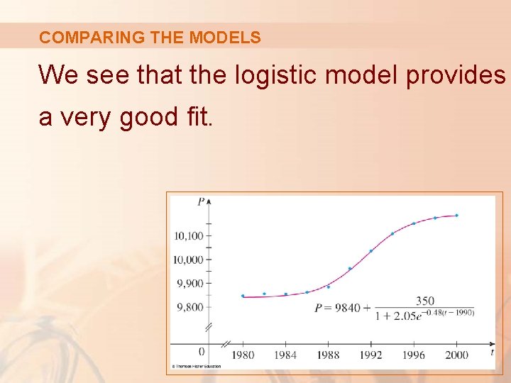
COMPARING THE MODELS This figure shows the data points of the table together with a shifted logistic function obtained from a calculator with the ability to fit a logistic function to these points by regression.

COMPARING THE MODELS We see that the logistic model provides a very good fit.

MODELS FOR POPULATION GROWTH The Law of Natural Growth and the logistic differential equation are not the only equations that have been proposed to model population growth.

OTHER MODELS FOR POPULATION GROWTH In Exercise 18, we look at the Gompertz growth function. In Exercises 19 and 20, we investigate seasonal-growth models.

OTHER MODELS FOR POPULATION GROWTH Two of the other models are modifications of the logistic model.

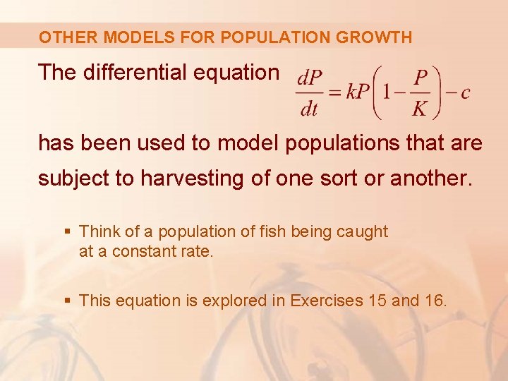
OTHER MODELS FOR POPULATION GROWTH The differential equation has been used to model populations that are subject to harvesting of one sort or another. § Think of a population of fish being caught at a constant rate. § This equation is explored in Exercises 15 and 16.

OTHER MODELS FOR POPULATION GROWTH For some species, there is a minimum population level m below which the species tends to become extinct. § Adults may not be able to find suitable mates.

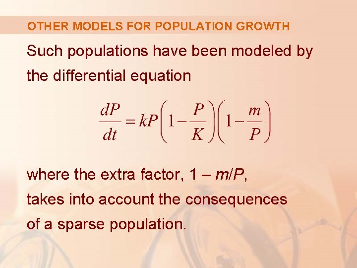
OTHER MODELS FOR POPULATION GROWTH Such populations have been modeled by the differential equation where the extra factor, 1 – m/P, takes into account the consequences of a sparse population.