GEOGG 121 Methods Differential Equations MC etc Dr

- Slides: 52

GEOGG 121: Methods Differential Equations, MC etc Dr. Mathias (Mat) Disney UCL Geography Office: 113, Pearson Building Tel: 7670 0592 Email: mathias. disney@ucl. ac. uk www. geog. ucl. ac. uk/~mdisney

Lecture outline • Differential equations – Introduction & importance – Types of DE • Examples • Solving ODEs – Analytical methods • General solution, particular solutions • Separation of variables, integrating factors, linear operators – Numerical methods • Euler, Runge-Kutta

Reading material • Textbooks These are good UG textbooks that have WAY more detail than we need – Boas, M. L. , 1985 (2 nd ed) Mathematical Methods in the Physical Sciences, Wiley, 793 pp. – Riley, K. F. , M. Hobson & S. Bence (2006) Mathematical Methods for Physics & Engineering, 3 rd ed. , CUP. – Croft, A. , Davison, R. & Hargreaves, M. (1996) Engineering Mathematics, 2 nd ed. , Addison Wesley. • Methods, applications – Wainwright, J. and M. Mulligan (eds, 2004) Environmental Modelling: Finding Simplicity in Complexity, J. Wiley and Sons, Chichester. Lots of examples particularly hydrology, soils, veg, climate. Useful intro. ch 1 on models and methods – Campbell, G. S. and J. Norman (1998) An Introduction to Environmental Biophysics, Springer NY, 2 nd ed. Excellent on applications eg Beer’s Law, heat transport etc. – Monteith, J. L. and M. H. Unsworth (1990) Principles of Environmental Physics, Edward Arnold. Small, but wide-ranging and superbly written. • Links – http: //www. math. ust. hk/~machas/differential-equations. pdf – http: //www. physics. ohio-state. edu/~physedu/mapletutorial/tutorials/diff_eqs/intro. html

Introduction • What is a differential equation? – General 1 st order DEs – 1 st case t is independent variable, x is dependent variable – 2 nd case, x is independent variable, y dependent • Extremely important – Equation relating rate of change of something (y) wrt to something else (x) – Any dynamic system (undergoing change) may be amenable to description by differential equations – Being able to formulate & solve is incredibly powerful

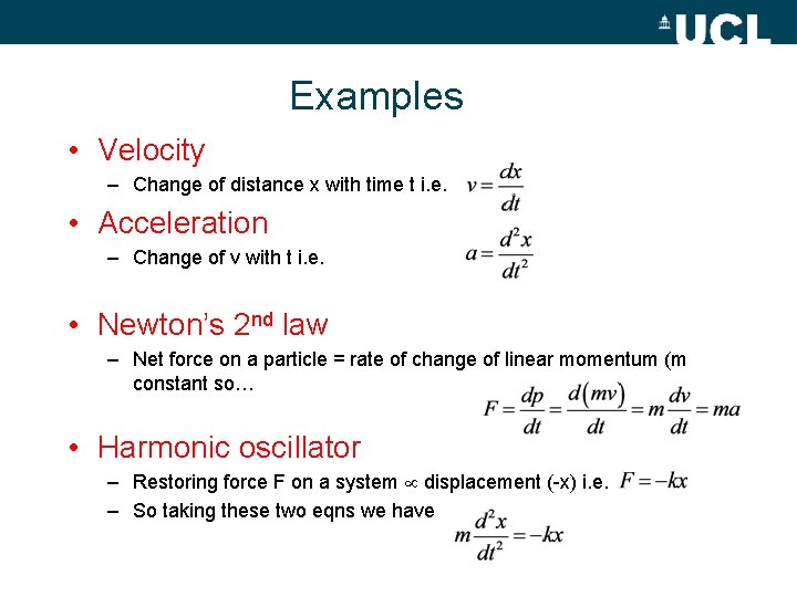
Examples • Velocity – Change of distance x with time t i. e. • Acceleration – Change of v with t i. e. • Newton’s 2 nd law – Net force on a particle = rate of change of linear momentum (m constant so… • Harmonic oscillator – Restoring force F on a system displacement (-x) i. e. – So taking these two eqns we have

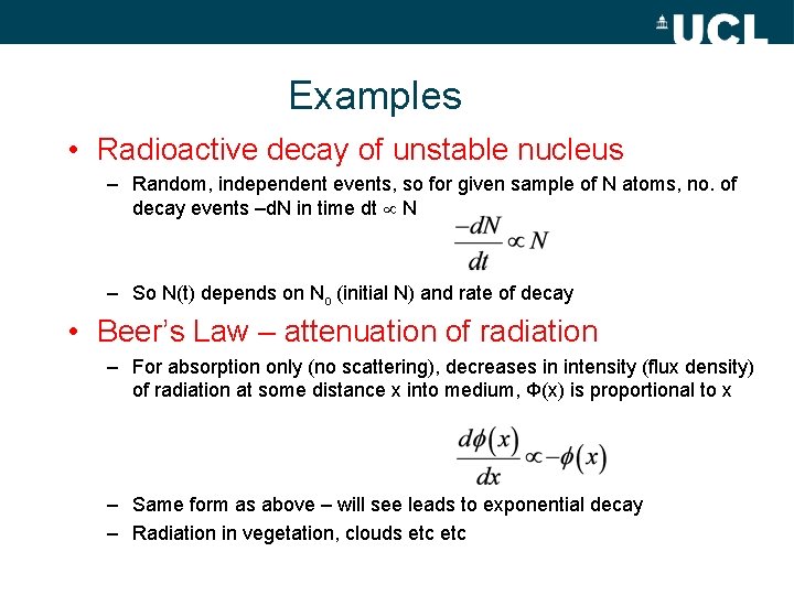
Examples • Radioactive decay of unstable nucleus – Random, independent events, so for given sample of N atoms, no. of decay events –d. N in time dt N – So N(t) depends on No (initial N) and rate of decay • Beer’s Law – attenuation of radiation – For absorption only (no scattering), decreases in intensity (flux density) of radiation at some distance x into medium, Φ(x) is proportional to x – Same form as above – will see leads to exponential decay – Radiation in vegetation, clouds etc

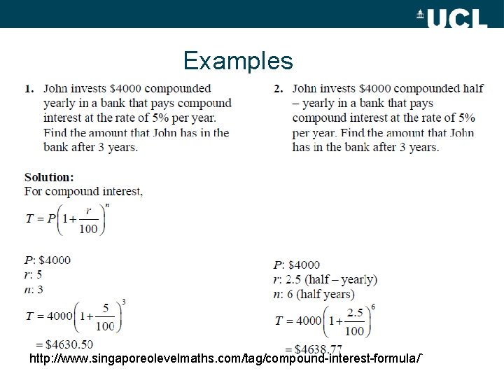
Examples • Compound Interest – How does an investment S(t), change with time, given an annual interest rate r compounded every time interval Δt, and annual deposit amount k? – Assuming deposit made after every time interval Δt – So as Δt 0 http: //www. thecreditexaminer. com/five-things-to-know-about-compound-interest-and-saving http: //www. singaporeolevelmaths. com/tag/compound-interest-formula/`

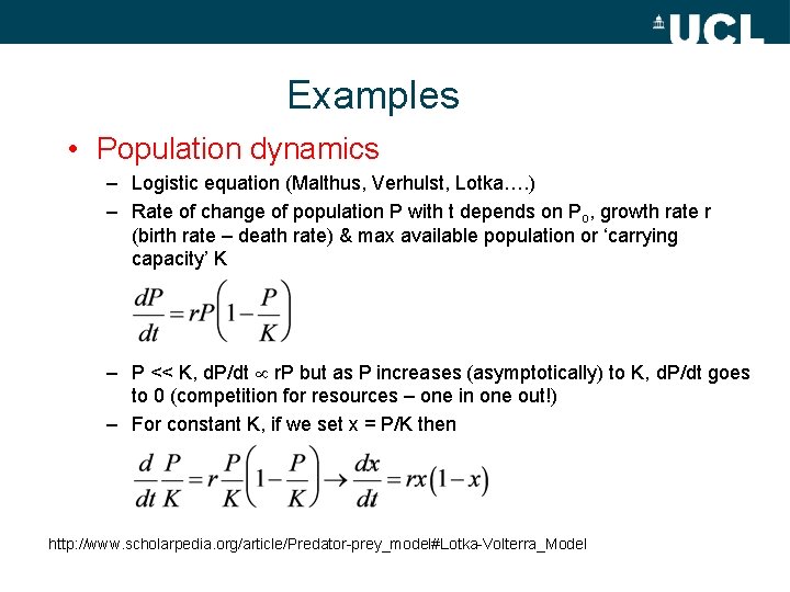
Examples • Population dynamics – Logistic equation (Malthus, Verhulst, Lotka…. ) – Rate of change of population P with t depends on Po, growth rate r (birth rate – death rate) & max available population or ‘carrying capacity’ K – P << K, d. P/dt r. P but as P increases (asymptotically) to K, d. P/dt goes to 0 (competition for resources – one in one out!) – For constant K, if we set x = P/K then http: //www. scholarpedia. org/article/Predator-prey_model#Lotka-Volterra_Model

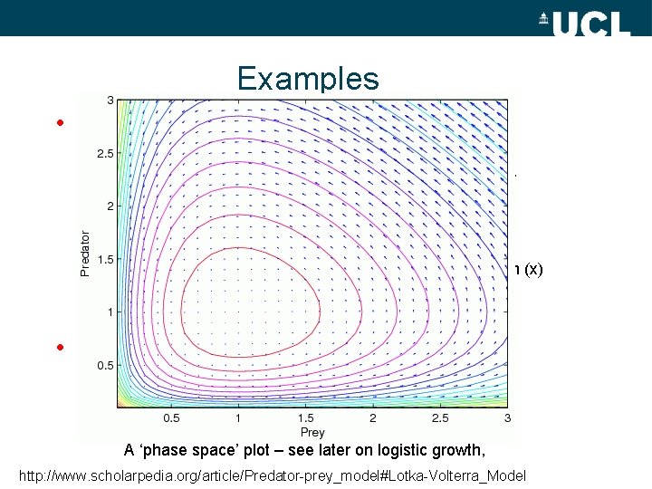
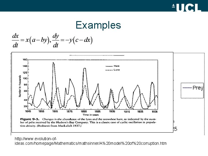
Examples • Population dynamics: II – Lotka-Volterra (predator-prey) equations – Same form, but now two populations x and y, with time – – y is predator and yt+1 depends on yt AND prey population (x) – x is prey, and xt+1 depends on xt AND y – a, b, c, d – parameters describing relationship of y to x • More generally can describe – Competition – eg economic modelling – Resources – reaction-diffusion equations A ‘phase space’ plot – see later on logistic growth, http: //www. scholarpedia. org/article/Predator-prey_model#Lotka-Volterra_Model

Examples http: //www. evolution-ofideas. com/homepage/Mathematics/mathsinner/A%20 model%20 of%20 corruption. htm

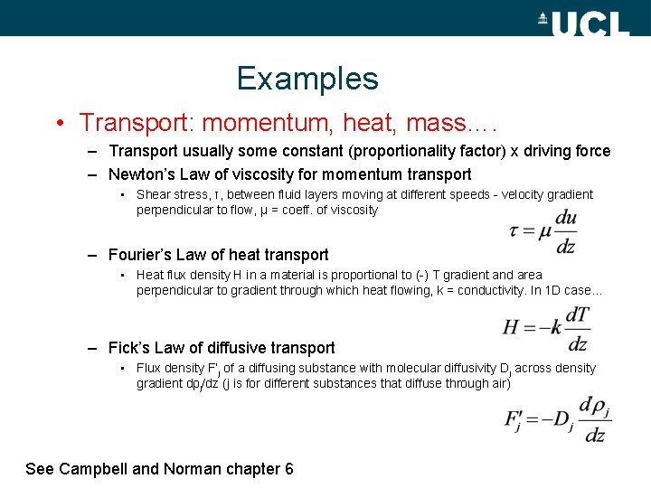
Examples • Transport: momentum, heat, mass…. – Transport usually some constant (proportionality factor) x driving force – Newton’s Law of viscosity for momentum transport • Shear stress, τ, between fluid layers moving at different speeds - velocity gradient perpendicular to flow, μ = coeff. of viscosity – Fourier’s Law of heat transport • Heat flux density H in a material is proportional to (-) T gradient and area perpendicular to gradient through which heat flowing, k = conductivity. In 1 D case… – Fick’s Law of diffusive transport • Flux density F’j of a diffusing substance with molecular diffusivity Dj across density gradient dρj/dz (j is for different substances that diffuse through air) See Campbell and Norman chapter 6

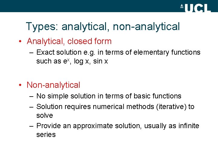
Types: analytical, non-analytical • Analytical, closed form – Exact solution e. g. in terms of elementary functions such as ex, log x, sin x • Non-analytical – No simple solution in terms of basic functions – Solution requires numerical methods (iterative) to solve – Provide an approximate solution, usually as infinite series

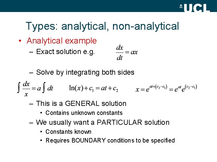
Types: analytical, non-analytical • Analytical example – Exact solution e. g. – Solve by integrating both sides – This is a GENERAL solution • Contains unknown constants – We usually want a PARTICULAR solution • Constants known • Requires BOUNDARY conditions to be specified

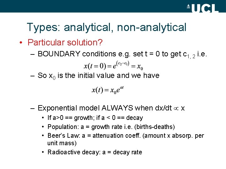
Types: analytical, non-analytical • Particular solution? – BOUNDARY conditions e. g. set t = 0 to get c 1, 2 i. e. – So x 0 is the initial value and we have – Exponential model ALWAYS when dx/dt x • If a>0 == growth; if a < 0 == decay • Population: a = growth rate i. e. (births-deaths) • Beer’s Law: a = attenuation coeff. (amount x absorp. per unit mass) • Radioactive decay: a = decay rate

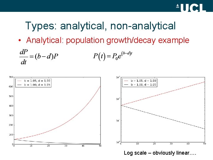
Types: analytical, non-analytical • Analytical: population growth/decay example Log scale – obviously linear….

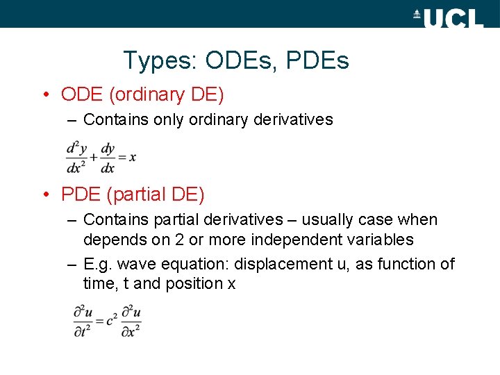
Types: ODEs, PDEs • ODE (ordinary DE) – Contains only ordinary derivatives • PDE (partial DE) – Contains partial derivatives – usually case when depends on 2 or more independent variables – E. g. wave equation: displacement u, as function of time, t and position x

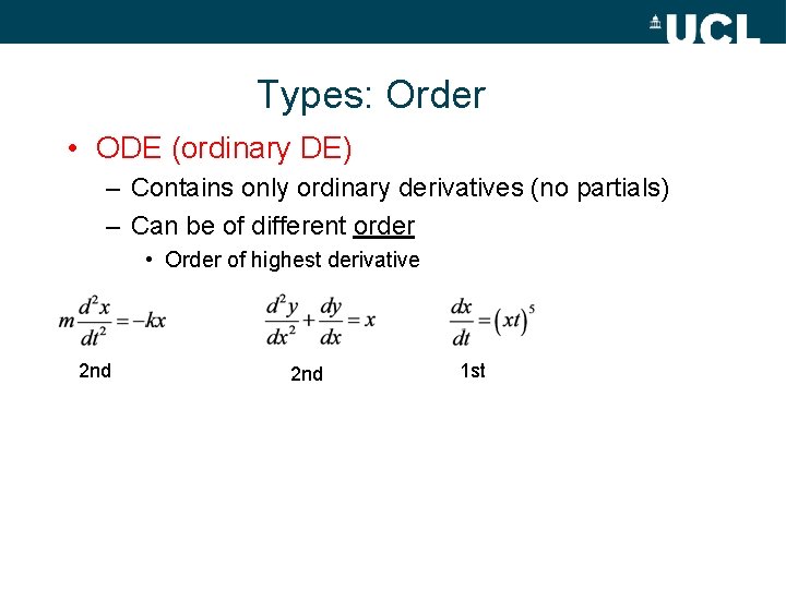
Types: Order • ODE (ordinary DE) – Contains only ordinary derivatives (no partials) – Can be of different order • Order of highest derivative 2 nd 1 st

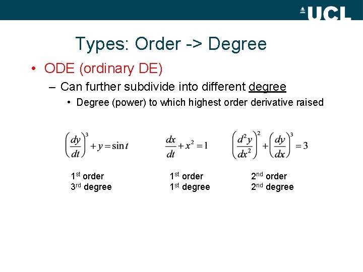
Types: Order -> Degree • ODE (ordinary DE) – Can further subdivide into different degree • Degree (power) to which highest order derivative raised 1 st order 3 rd degree 1 st order 1 st degree 2 nd order 2 nd degree

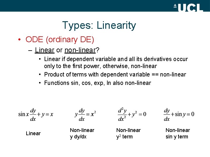
Types: Linearity • ODE (ordinary DE) – Linear or non-linear? • Linear if dependent variable and all its derivatives occur only to the first power, otherwise, non-linear • Product of terms with dependent variable == non-linear • Functions sin, cos, exp, ln also non-linear Linear Non-linear y dy/dx Non-linear y 2 term Non-linear sin y term

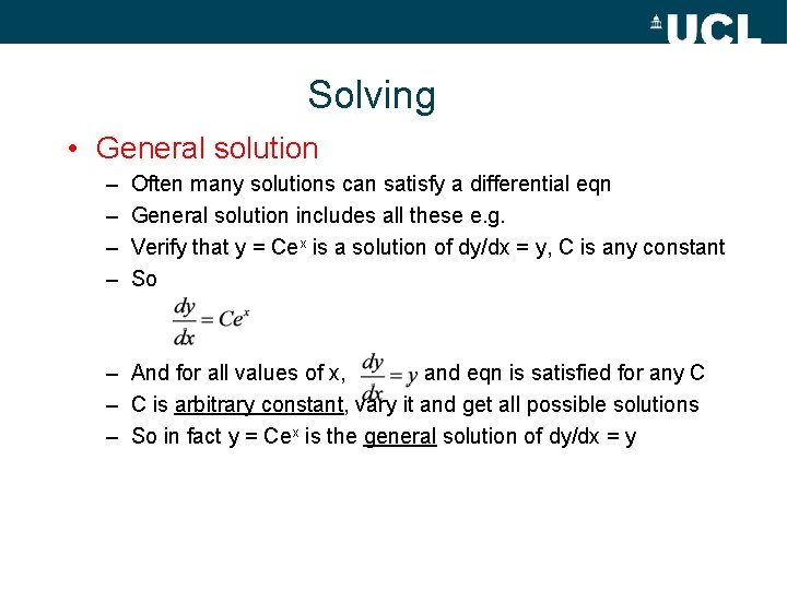
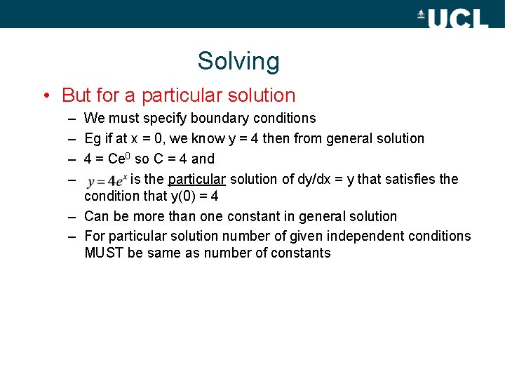
Solving • General solution – – Often many solutions can satisfy a differential eqn General solution includes all these e. g. Verify that y = Cex is a solution of dy/dx = y, C is any constant So – And for all values of x, and eqn is satisfied for any C – C is arbitrary constant, vary it and get all possible solutions – So in fact y = Cex is the general solution of dy/dx = y

Solving • But for a particular solution – We must specify boundary conditions – Eg if at x = 0, we know y = 4 then from general solution – 4 = Ce 0 so C = 4 and – is the particular solution of dy/dx = y that satisfies the condition that y(0) = 4 – Can be more than one constant in general solution – For particular solution number of given independent conditions MUST be same as number of constants

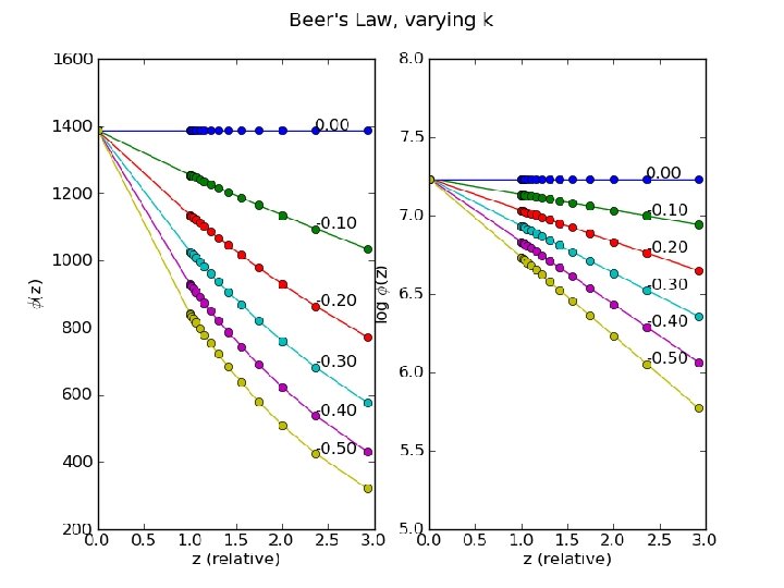
Types: analytical, non-analytical • Analytical: Beer’s Law - attenuation – k is extinction coefficient – absorptivity per unit depth, z (m-1) – E. g. attenuation through atmosphere, where path length (z) 1/cos(θsun), θsun is the solar zenith angle – Take logs: – Plot z against ln(ϕ), slope is k, intercept is ϕ 0 i. e. solar radiation with no attenuation (top of atmos. – solar constant) – [NB taking logs v powerful – always linearise if you can!]

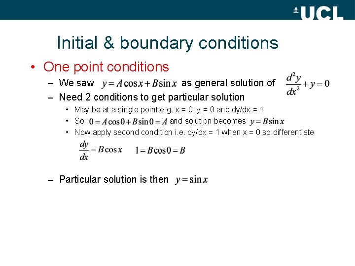
Initial & boundary conditions • One point conditions – We saw as general solution of – Need 2 conditions to get particular solution • May be at a single point e. g. x = 0, y = 0 and dy/dx = 1 • So and solution becomes • Now apply secondition i. e. dy/dx = 1 when x = 0 so differentiate – Particular solution is then

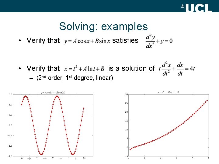
Solving: examples • Verify that satisfies is a solution of – (2 nd order, 1 st degree, linear)

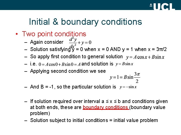
Initial & boundary conditions • Two point conditions – – – Again consider Solution satisfying y = 0 when x = 0 AND y = 1 when x = 3π/2 So apply first condition to general solution i. e. and solution is Applying secondition we see – And B = -1, so the particular solution is – If solution required over interval a ≤ x ≤ b and conditions given at both ends, these are boundary conditions (boundary value problem) – Solution subject to initial conditions = initial value problem

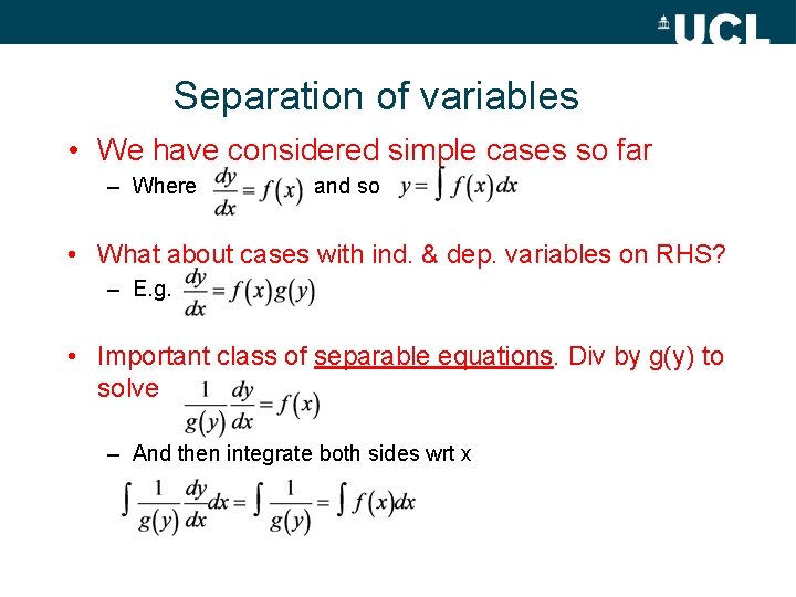
Separation of variables • We have considered simple cases so far – Where and so • What about cases with ind. & dep. variables on RHS? – E. g. • Important class of separable equations. Div by g(y) to solve – And then integrate both sides wrt x

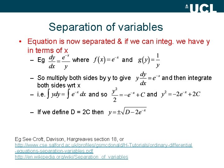
Separation of variables • Equation is now separated & if we can integ. we have y in terms of x – Eg where and – So multiply both sides by y to give both sides wrt x – i. e. and so and then integrate and – If we define D = 2 C then Eg See Croft, Davison, Hargreaves section 18, or http: //www. cse. salford. ac. uk/profiles/gsmcdonald/H-Tutorials/ordinary-differential -equations-separation-variables. pdf http: //en. wikipedia. org/wiki/Separation_of_variables

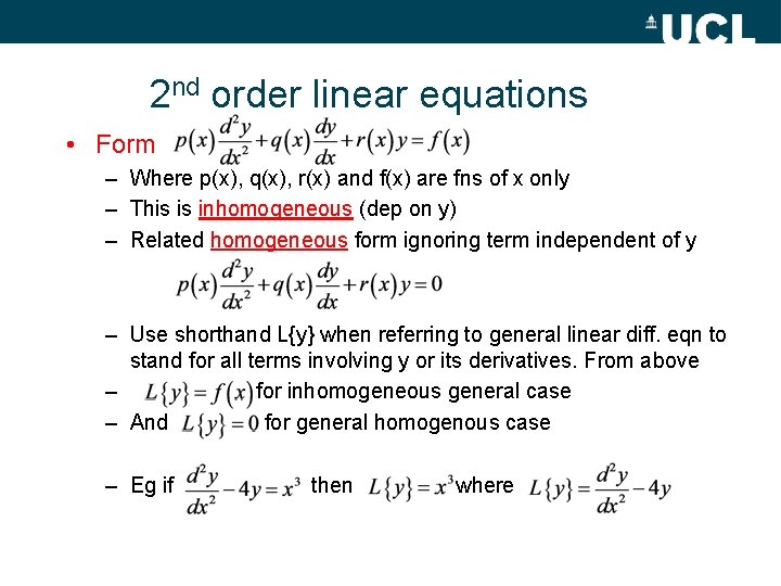
2 nd order linear equations • Form – Where p(x), q(x), r(x) and f(x) are fns of x only – This is inhomogeneous (dep on y) – Related homogeneous form ignoring term independent of y – Use shorthand L{y} when referring to general linear diff. eqn to stand for all terms involving y or its derivatives. From above – for inhomogeneous general case – And for general homogenous case – Eg if then where

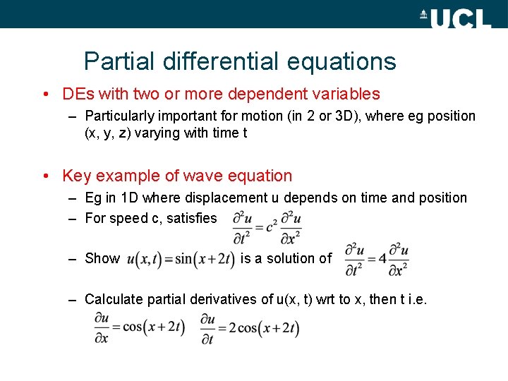
Partial differential equations • DEs with two or more dependent variables – Particularly important for motion (in 2 or 3 D), where eg position (x, y, z) varying with time t • Key example of wave equation – Eg in 1 D where displacement u depends on time and position – For speed c, satisfies – Show is a solution of – Calculate partial derivatives of u(x, t) wrt to x, then t i. e.

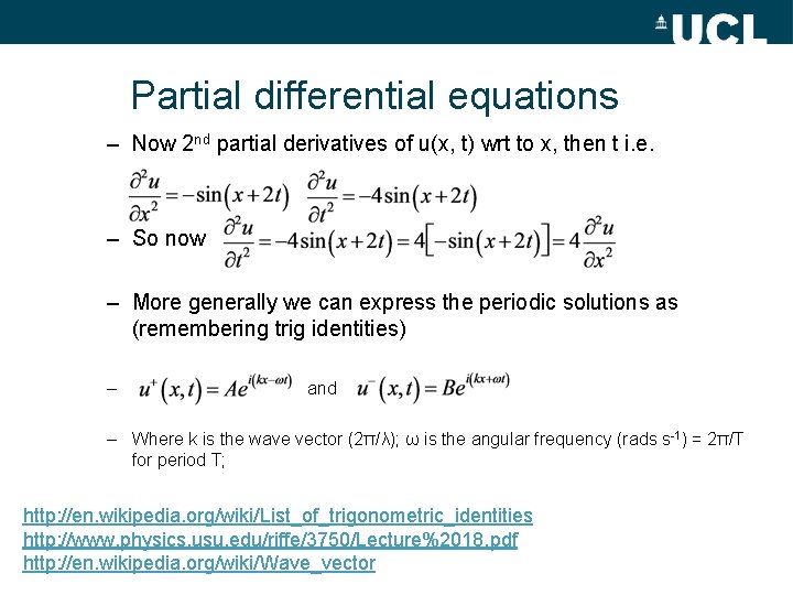
Partial differential equations – Now 2 nd partial derivatives of u(x, t) wrt to x, then t i. e. – So now – More generally we can express the periodic solutions as (remembering trig identities) – and – Where k is the wave vector (2π/λ); ω is the angular frequency (rads s-1) = 2π/T for period T; http: //en. wikipedia. org/wiki/List_of_trigonometric_identities http: //www. physics. usu. edu/riffe/3750/Lecture%2018. pdf http: //en. wikipedia. org/wiki/Wave_vector

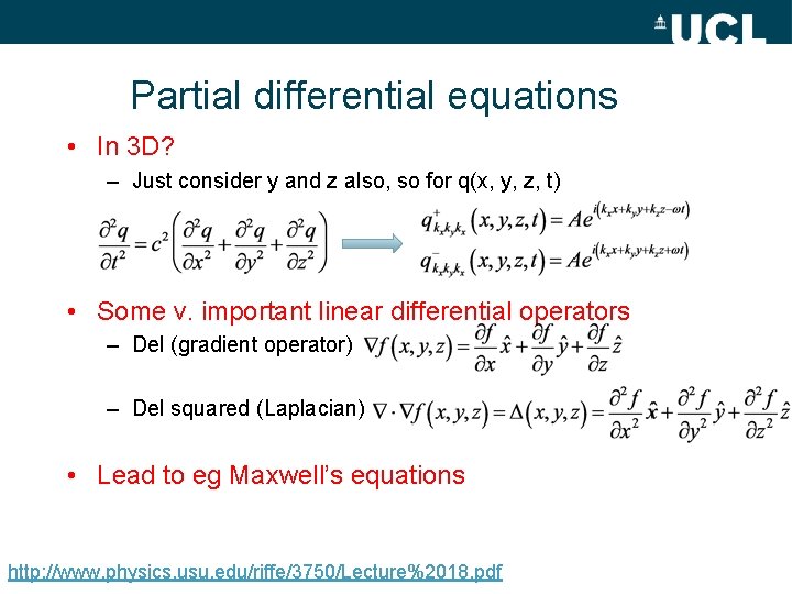
Partial differential equations • In 3 D? – Just consider y and z also, so for q(x, y, z, t) • Some v. important linear differential operators – Del (gradient operator) – Del squared (Laplacian) • Lead to eg Maxwell’s equations http: //www. physics. usu. edu/riffe/3750/Lecture%2018. pdf

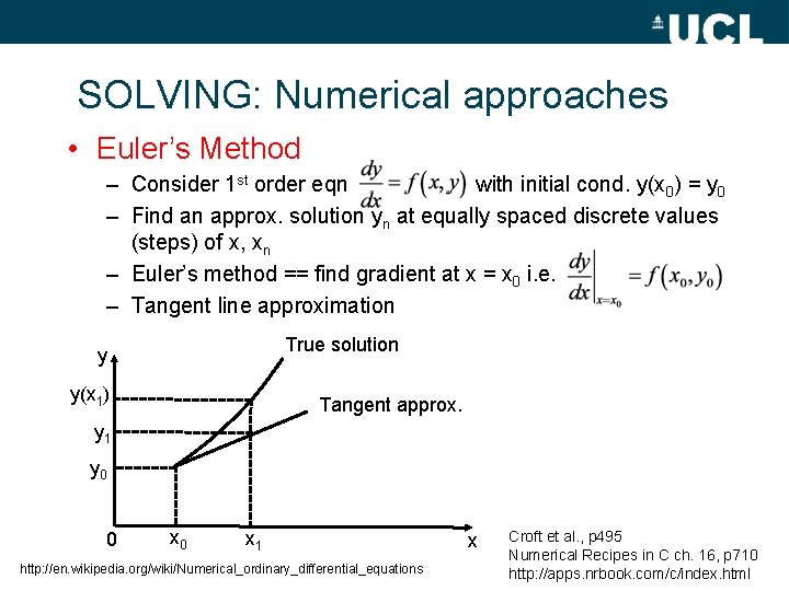
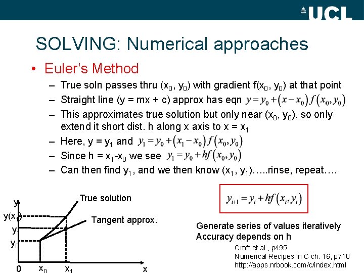
SOLVING: Numerical approaches • Euler’s Method – Consider 1 st order eqn with initial cond. y(x 0) = y 0 – Find an approx. solution yn at equally spaced discrete values (steps) of x, xn – Euler’s method == find gradient at x = x 0 i. e. – Tangent line approximation True solution y y(x 1) Tangent approx. y 1 y 0 0 x 1 http: //en. wikipedia. org/wiki/Numerical_ordinary_differential_equations x Croft et al. , p 495 Numerical Recipes in C ch. 16, p 710 http: //apps. nrbook. com/c/index. html

SOLVING: Numerical approaches • Euler’s Method – True soln passes thru (x 0, y 0) with gradient f(x 0, y 0) at that point – Straight line (y = mx + c) approx has eqn – This approximates true solution but only near (x 0, y 0), so only extend it short dist. h along x axis to x = x 1 – Here, y = y 1 and – Since h = x 1 -x 0 we see – Can then find y 1, and we then know (x 1, y 1)…. . rinse, repeat…. True solution y y(x 1) y 1 y 0 0 Tangent approx. x x x Generate series of values iteratively Accuracy depends on h Croft et al. , p 495 Numerical Recipes in C ch. 16, p 710 http: //apps. nrbook. com/c/index. html

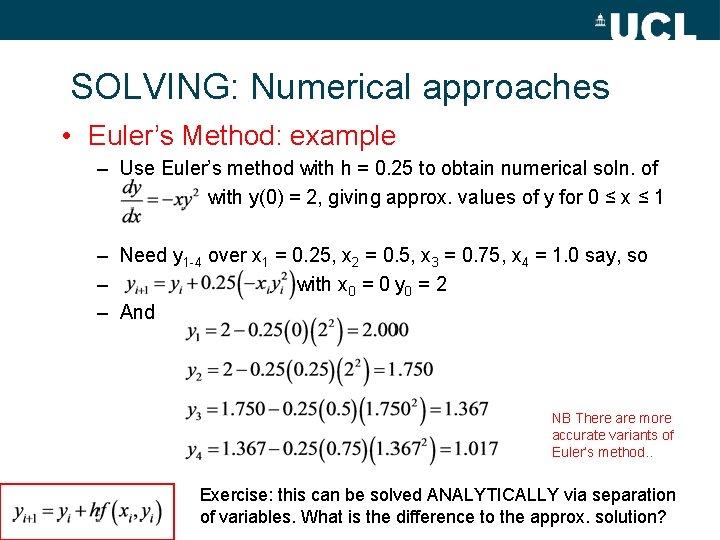
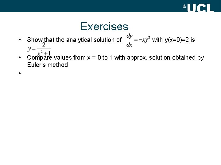
SOLVING: Numerical approaches • Euler’s Method: example – Use Euler’s method with h = 0. 25 to obtain numerical soln. of with y(0) = 2, giving approx. values of y for 0 ≤ x ≤ 1 – Need y 1 -4 over x 1 = 0. 25, x 2 = 0. 5, x 3 = 0. 75, x 4 = 1. 0 say, so – with x 0 = 0 y 0 = 2 – And NB There are more accurate variants of Euler’s method. . Exercise: this can be solved ANALYTICALLY via separation of variables. What is the difference to the approx. solution?

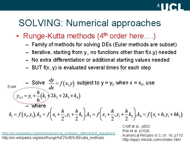
SOLVING: Numerical approaches • Runge-Kutta methods (4 th order here…. ) – – Euler Family of methods for solving DEs (Euler methods are subset) Iterative, starting from yi, no functions other than f(x, y) needed No extra differentiation or additional starting values needed BUT f(x, y) is evaluated several times for each step – Solve subject to y = y 0 when x = x 0, use – where http: //en. wikipedia. org/wiki/Numerical_ordinary_differential_equations http: //en. wikipedia. org/wiki/Runge%E 2%80%93 Kutta_methods Croft et al. , p 502 Rile et al. p 1026 Numerical Recipes in C ch. 16, p 710 http: //apps. nrbook. com/c/index. html

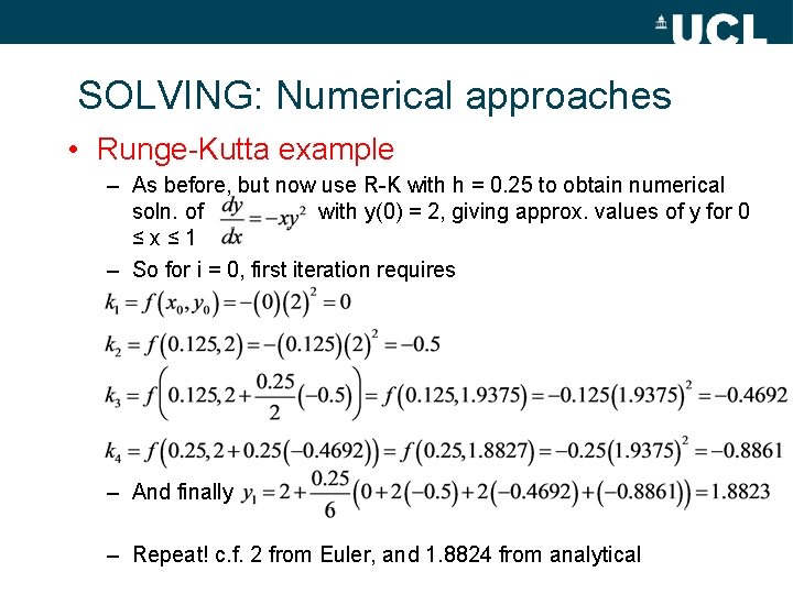
SOLVING: Numerical approaches • Runge-Kutta example – As before, but now use R-K with h = 0. 25 to obtain numerical soln. of with y(0) = 2, giving approx. values of y for 0 ≤x≤ 1 – So for i = 0, first iteration requires – And finally – Repeat! c. f. 2 from Euler, and 1. 8824 from analytical

Very brief intro to Monte Carlo • Brute force method(s) for integration / parameter estimation / sampling – Powerful BUT essentially last resort as involves random sampling of parameter space – Time consuming – more samples gives better approximation – Errors tend to reduce as 1/N 1/2 • N = 100 -> error down by 10; N = 1000000 -> error down by 1000 – Fast computers can solve complex problems • Applications: – Numerical integration (eg radiative transfer eqn), Bayesian inference, computational physics, sensitivity analysis etc http: //en. wikipedia. org/wiki/Monte_Carlo_method http: //en. wikipedia. org/wiki/Monte_Carlo_integration Numerical Recipes in C ch. 7, p 304 http: //apps. nrbook. com/c/index. html

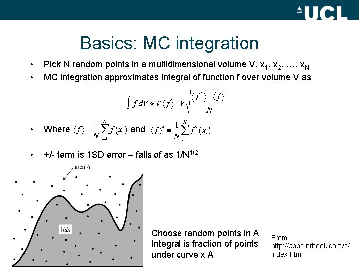
Basics: MC integration • • Pick N random points in a multidimensional volume V, x 1, x 2, …. x. N MC integration approximates integral of function f over volume V as • Where • +/- term is 1 SD error – falls of as 1/N 1/2 and Choose random points in A Integral is fraction of points under curve x A From http: //apps. nrbook. com/c/ index. html

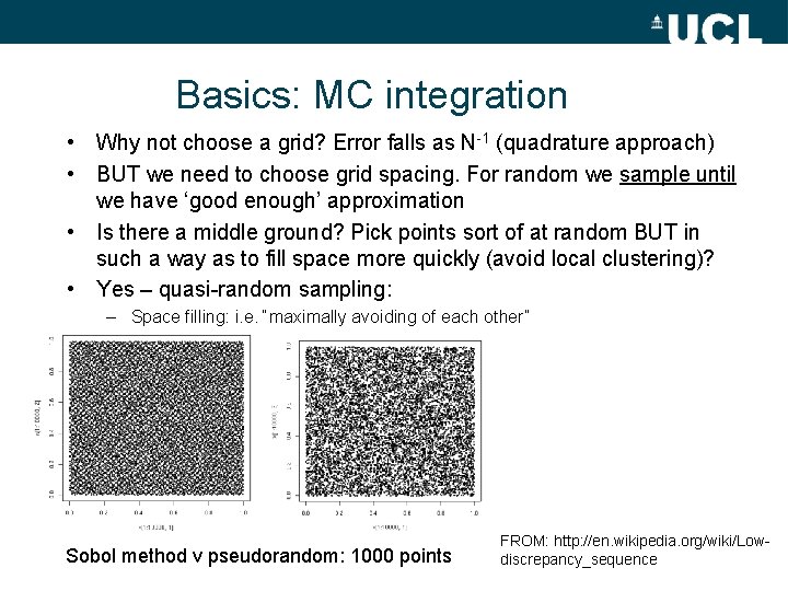
Basics: MC integration • Why not choose a grid? Error falls as N-1 (quadrature approach) • BUT we need to choose grid spacing. For random we sample until we have ‘good enough’ approximation • Is there a middle ground? Pick points sort of at random BUT in such a way as to fill space more quickly (avoid local clustering)? • Yes – quasi-random sampling: – Space filling: i. e. “maximally avoiding of each other” Sobol method v pseudorandom: 1000 points FROM: http: //en. wikipedia. org/wiki/Lowdiscrepancy_sequence

Summary • Differential equations – Describe dynamic systems – wide range of examples, particularly motion, population, decay (radiation – Beer’s Law, mass – radioactivity) • Types – – Analytical, closed form solution, simple functions Non-analytical: no simple solution, approximations? ODEs, PDEs Order: highest power of derivative • Degree: power to which highest order derivative is raised – Linear/non: • Linear if dependent variable and all its derivatives occur only to the first power, otherwise, non-linear

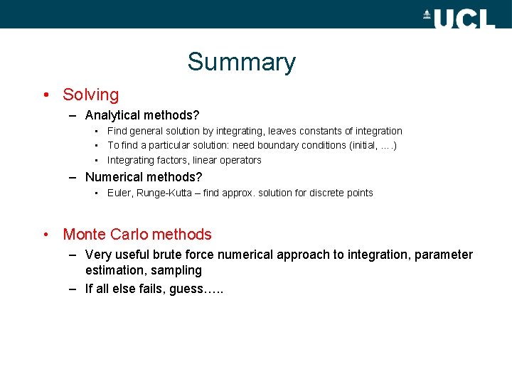
Summary • Solving – Analytical methods? • Find general solution by integrating, leaves constants of integration • To find a particular solution: need boundary conditions (initial, …. ) • Integrating factors, linear operators – Numerical methods? • Euler, Runge-Kutta – find approx. solution for discrete points • Monte Carlo methods – Very useful brute force numerical approach to integration, parameter estimation, sampling – If all else fails, guess…. .

END

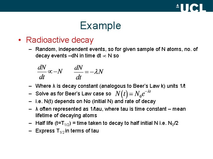
Example • Radioactive decay – Random, independent events, so for given sample of N atoms, no. of decay events –d. N in time dt N so – – Where λ is decay constant (analogous to Beer’s Law k) units 1/t Solve as for Beer’s Law case so i. e. N(t) depends on No (initial N) and rate of decay λ often represented as 1/tau, where tau is time constant – mean lifetime of decaying atoms – Half life (t=T 1/2) = time taken to decay to half initial N i. e. N 0/2 – Express T 1/2 in terms of tau

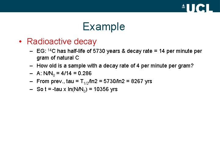
Example • Radioactive decay – EG: 14 C has half-life of 5730 years & decay rate = 14 per minute per gram of natural C – How old is a sample with a decay rate of 4 per minute per gram? – A: N/N 0 = 4/14 = 0. 286 – From prev. , tau = T 1/2/ln 2 = 5730/ln 2 = 8267 yrs – So t = -tau x ln(N/N 0) = 10356 yrs

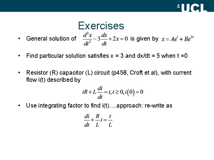
Exercises • General solution of is given by • Find particular solution satisfies x = 3 and dx/dt = 5 when t =0 • Resistor (R) capacitor (L) circuit (p 458, Croft et al), with current flow i(t) described by • Use integrating factor to find i(t)…. approach: re-write as

Exercises • Show that the analytical solution of with y(x=0)=2 is • Compare values from x = 0 to 1 with approx. solution obtained by Euler’s method •

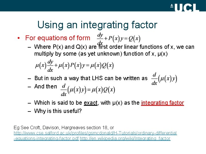
Using an integrating factor • For equations of form – Where P(x) and Q(x) are first order linear functions of x, we can multiply by some (as yet unknown) function of x, μ(x) – But in such a way that LHS can be written as – And then – Which is said to be exact, with μ(x) as the integrating factor – Why is this useful? Eg See Croft, Davison, Hargreaves section 18, or http: //www. cse. salford. ac. uk/profiles/gsmcdonald/H-Tutorials/ordinary-differential -equations-integrating-factor. pdf http: //en. wikipedia. org/wiki/Integrating_factor

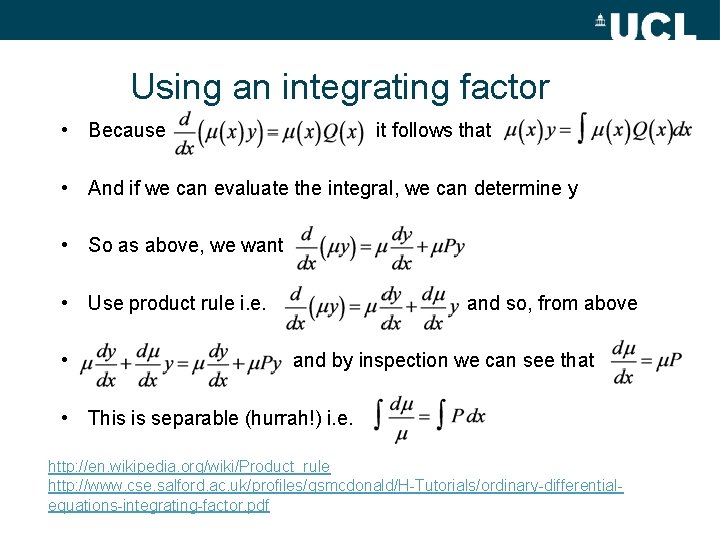
Using an integrating factor • Because it follows that • And if we can evaluate the integral, we can determine y • So as above, we want • Use product rule i. e. • and so, from above and by inspection we can see that • This is separable (hurrah!) i. e. http: //en. wikipedia. org/wiki/Product_rule http: //www. cse. salford. ac. uk/profiles/gsmcdonald/H-Tutorials/ordinary-differentialequations-integrating-factor. pdf

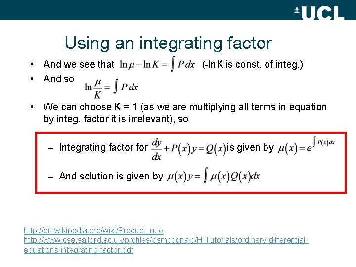
Using an integrating factor • And we see that • And so (-ln. K is const. of integ. ) • We can choose K = 1 (as we are multiplying all terms in equation by integ. factor it is irrelevant), so – Integrating factor for is given by – And solution is given by http: //en. wikipedia. org/wiki/Product_rule http: //www. cse. salford. ac. uk/profiles/gsmcdonald/H-Tutorials/ordinary-differentialequations-integrating-factor. pdf

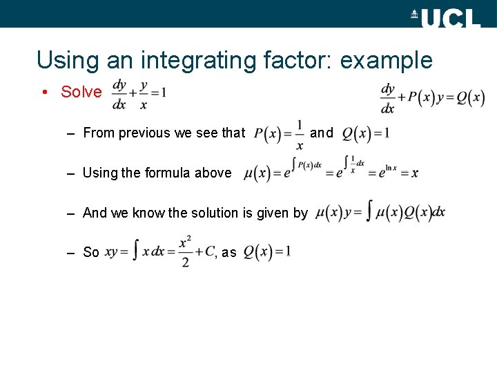
Using an integrating factor: example • Solve – From previous we see that – Using the formula above – And we know the solution is given by – So , as and

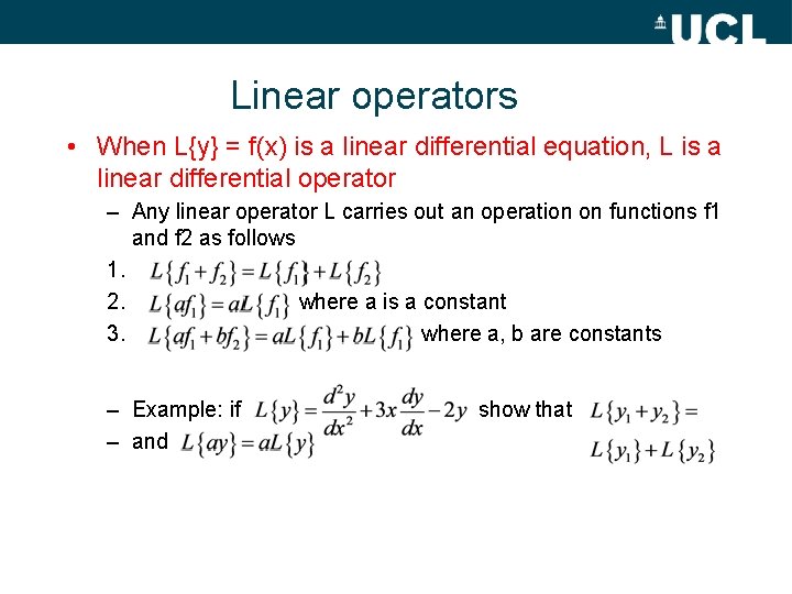
Linear operators • When L{y} = f(x) is a linear differential equation, L is a linear differential operator – Any linear operator L carries out an operation on functions f 1 and f 2 as follows 1. 2. where a is a constant 3. where a, b are constants – Example: if – and show that

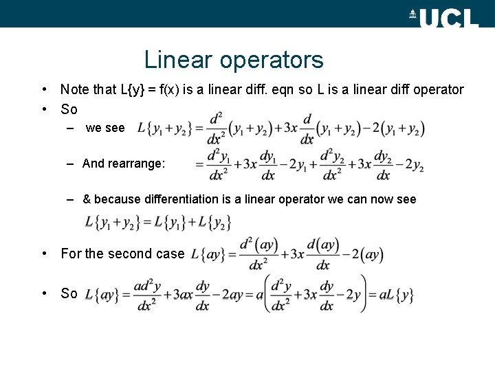
Linear operators • Note that L{y} = f(x) is a linear diff. eqn so L is a linear diff operator • So – we see – And rearrange: – & because differentiation is a linear operator we can now see • For the second case • So