GEOGG 121 Methods Monte Carlo methods revision Dr

GEOGG 121: Methods Monte Carlo methods, revision Dr. Mathias (Mat) Disney UCL Geography Office: 113, Pearson Building Tel: 7670 0592 Email: mdisney@ucl. geog. ac. uk www. geog. ucl. ac. uk/~mdisney

Very brief intro to Monte Carlo • Brute force method(s) for integration / parameter estimation / sampling – Powerful BUT essentially last resort as involves random sampling of parameter space – Time consuming – more samples gives better approximation – Errors tend to reduce as 1/N 1/2 • N = 100 -> error down by 10; N = 1000000 -> error down by 1000 – Fast computers can solve complex problems • Applications: – Numerical integration (eg radiative transfer eqn), Bayesian inference (posterior), computational physics, sensitivity analysis etc http: //en. wikipedia. org/wiki/Monte_Carlo_method http: //en. wikipedia. org/wiki/Monte_Carlo_integration Numerical Recipes in C ch. 7, p 304 http: //apps. nrbook. com/c/index. html

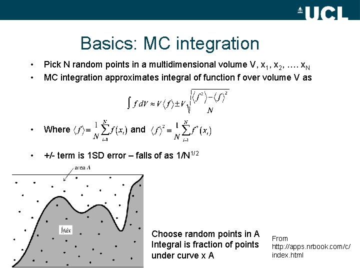
Basics: MC integration • • Pick N random points in a multidimensional volume V, x 1, x 2, …. x. N MC integration approximates integral of function f over volume V as • Where • +/- term is 1 SD error – falls of as 1/N 1/2 and Choose random points in A Integral is fraction of points under curve x A From http: //apps. nrbook. com/c/ index. html

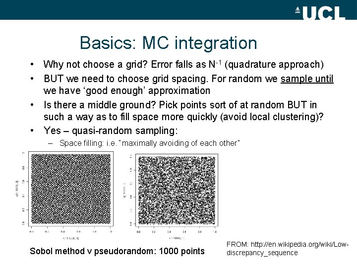
Basics: MC integration • Why not choose a grid? Error falls as N-1 (quadrature approach) • BUT we need to choose grid spacing. For random we sample until we have ‘good enough’ approximation • Is there a middle ground? Pick points sort of at random BUT in such a way as to fill space more quickly (avoid local clustering)? • Yes – quasi-random sampling: – Space filling: i. e. “maximally avoiding of each other” Sobol method v pseudorandom: 1000 points FROM: http: //en. wikipedia. org/wiki/Lowdiscrepancy_sequence

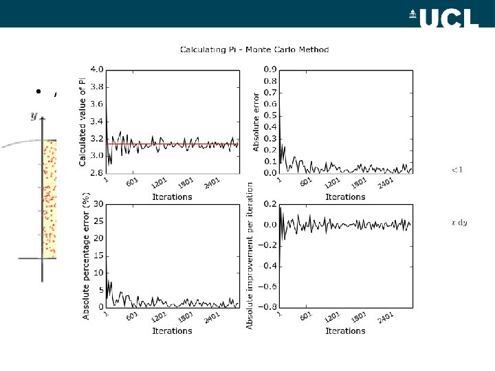
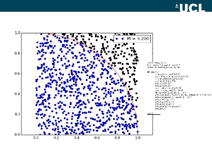
MC approximation of Pi? • A simple example of MC methods in practice

MC approximation of Pi? • A simple example of MC methods in practice • In Python? – – import numpy as np a = np. random. rand(10, 2) np. sum(a*a, 1)<1 array([ True, False, True, True], dtype=bool) – 4*np. mean(np. sum(a*a, 1)<1) 2. 399999999

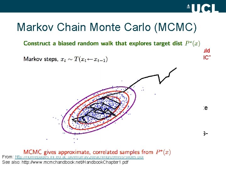
Markov Chain Monte Carlo (MCMC) • Integration / parameter estimation / sampling – From 80 s: “It was rapidly realised that most Bayesian inference could be done by MCMC, whereas very little could be done without MCMC” (Geyer, 2010) • Formally – MCMC methods sample from probability distribution (eg a posterior) based on constructing a Markov Chain with the desired distribution as its equilibrium (tends to) distribution – Markov Chain: system of random transitions where next state dpeends on only on current, not preceding chain (ie no “memory” of how we got here) • Many implementations of MCMC including Metropolis. Hastings, Gibbs Sampler etc. From: http: //homepages. inf. ed. ac. uk/imurray 2/teaching/09 mlss/slides. pdf See also: http: //www. mcmchandbook. net/Handbook. Chapter 1. pdf

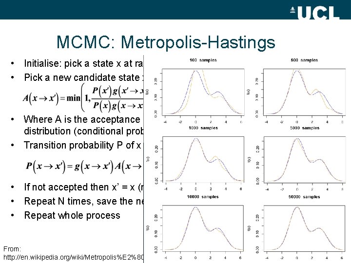
MCMC: Metropolis-Hastings • Initialise: pick a state x at random • Pick a new candidate state x’ at random. Accept based on criteria • Where A is the acceptance distribution, is the proposal distribution (conditional prob of proposing state x’, given x) • Transition probability P of x -> x’ • If not accepted then x’ = x (no change) OR state transits to x’ • Repeat N times, save the new state x’ • Repeat whole process From: http: //en. wikipedia. org/wiki/Metropolis%E 2%80

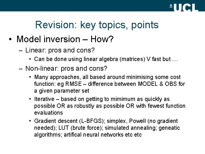
Revision: key topics, points • Model inversion – why? – Forward model: model predicts system behaviour based on given set of parameter values (system state vector) f(x) – BUT we usually want to observe system and INFER parameter values – Inversion: f-1(x) - estimate the parameter values (system state) that give rise to observed values – Forward modelling useful for understanding system, sensitivity analysis etc. – Inverse model allows us to estimate system state

Revision: key topics, points • Model inversion – How? – Linear: pros and cons? • Can be done using linear algebra (matrices) V fast but … – Non-linear: pros and cons? • Many approaches, all based around minimising some cost function: eg RMSE – difference between MODEL & OBS for a given parameter set • Iterative – based on getting to mimimum as quickly as possible OR as robustly as possible OR with fewest function evaluations • Gradient descent (L-BFGS); simplex, Powell (no gradient needed); LUT (brute force); simulated annealing; geneatic algorithms; artifical neural networks etc

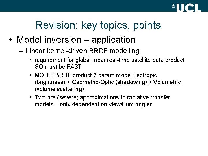
Revision: key topics, points • Model inversion – application – Linear kernel-driven BRDF modelling • requirement for global, near real-time satellite data product SO must be FAST • MODIS BRDF product 3 param model: Isotropic (brightness) + Geometric-Optic (shadowing) + Volumetric (volume scattering) • Two are (severe) approximations to radiative transfer models – only dependent on view/illum angles

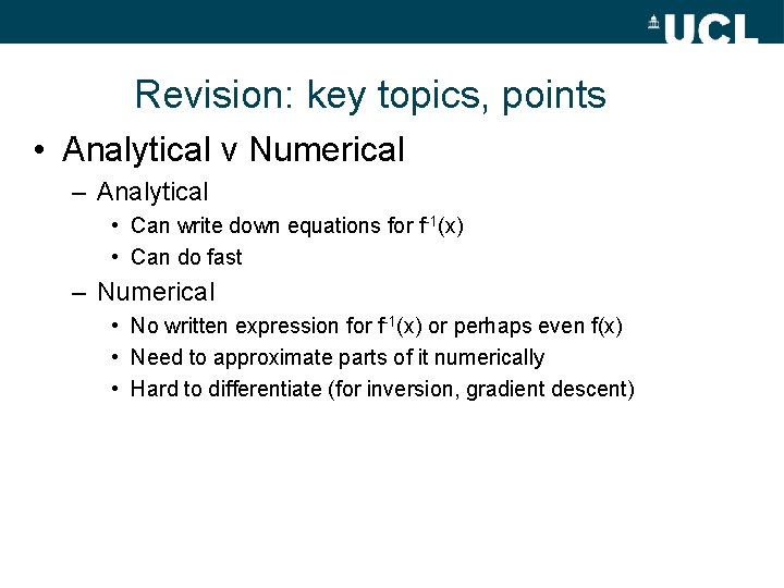
Revision: key topics, points • Analytical v Numerical – Analytical • Can write down equations for f-1(x) • Can do fast – Numerical • No written expression for f-1(x) or perhaps even f(x) • Need to approximate parts of it numerically • Hard to differentiate (for inversion, gradient descent)