GEOGG 121 Methods Inversion II nonlinear methods Dr

GEOGG 121: Methods Inversion II: non-linear methods Dr. Mathias (Mat) Disney UCL Geography Office: 113, Pearson Building Tel: 7670 0592 Email: mdisney@ucl. geog. ac. uk www. geog. ucl. ac. uk/~mdisney

Lecture outline • Non-linear models, inversion – – – The non-linear problem Parameter estimation, uncertainty Numerical approaches Implementation Practical examples

Reading • Non-linear models, inversion – Gradient descent: Press et al. Numerical Recipes in C (1992) online version), Section 10. 7 eg BFGS http: //apps. nrbook. com/c/index. html – Conjugate gradient, Simplex, Simulated Annealing etc. : Press et al. Numerical Recipes in C (1992), ch. 10 http: //apps. nrbook. com/c/index. html – Liang, S. (2004) Quantitative Remote Sensing of the Land Surface, ch. 8 (section 8. 2). – Gershenfeld, N. (2002) The Nature of Mathematical Modelling, CUP

Non-linear inversion • If we cannot phrase our problem in linear form, then we have non-linear inversion problem • Key tool for many applications – Resource allocation – Systems control – (Non-linear) Model parameter estimation • AKA curve or function fitting: i. e. obtain parameter values that provide “best fit” (in some sense) to a set of observations • And estimate of parameter uncertainty, model fit 4

Options for Numerical Inversion • Same principle as for linear – i. e. find minimum of some cost func. expressing difference between model and obs – We want some set of parameters (x*) which minimise cost function f(x) i. e. for some (small) tolerance δ > 0 so for all x – Where f(x*) ≤ f(x). So for some region around x*, all values of f(x) are higher (a local minima – may be many) – If region encompasses full range of x, then we have the global minima

Numerical Inversion • Iterative numerical techniques – Can we differentiate model (e. g. adjoint)? – YES: Quasi-Newton (eg BFGS etc) – NO: Powell, Simplex, Simulated annealing, Artificial Neural Networks (ANNs), Genetic Algorithms (GAs), Look-up Tables (LUTs); Knowledge-based systems (KBS) Errico (1997) What is an adjoint model? , BAMS, 78, 2577 -2591 http: //paoc 2001. mit. edu/cmi/development/adjoint. htm

Today • Outline principle of Quasi-Newton: – BFGS • Outline principles when no differential: – Powell, Simplex, Simulated annealing • V. briefly mention: – Artificial Neural Networks (ANNs) – Look-up Tables (LUTs) – v. useful brute force method Errico (1997) What is an adjoint model? , BAMS, 78, 2577 -2591 http: //paoc 2001. mit. edu/cmi/development/adjoint. htm

First order optimisation: gradient descent • For multivariate function F(x) in neighbourhood of point a, F(x) decreases fastest if we move in direction of –ve gradient i. e. • If for small enough step size γ, then F(a) ≥ F(b) • And for sequence x 0, x 1, x 2 … xn we have http: //en. wikipedia. org/wiki/Gradient_descent

Newton’s method • Construct a sequence xn starting at x 0, converging to x* where f’(x*) = 0, the stationary point of f(x), by approximating as a quadratic…. • 2 nd order Taylor expansion around xn (where Δx= x – xn) is • Max where d(Δx)/dx = 0 i. e. for linear eqn • So for sequence xn • So http: //en. wikipedia. org/wiki/Newton%27 s_method_in_optimization Red: Newton green: grad. descent

Quasi-Newton methods… • Quasi-Newton: use Taylor approx also, but Hessian matrix of 2 nd derivatives doesn’t need to be computed • Update Hessian by analysing successive derivatives instead • • • Where is the gradient and B is approx. to Hessian matrix So gradient of this approx is So set to zero i. e. And choose B (Hessian approx. ) to satisfy Various methods to choose/update B – eg BFGS (Broyden-Fletcher-Goldfarb-Shanno) – Iterative line searches using approx. to 2 nd differential http: //en. wikipedia. org/wiki/Quasi-Newton_method http: //en. wikipedia. org/wiki/BFGS_method

Methods without derivatives: local and global minima (general: optima) Need starting point

How to go ‘downhill’? Bracketing of a minimum: choose new points at each end closer to a minimum

Slow, but sure How far to go ‘downhill’? i. e. how to choose next points? w=(b-a)/(c-a) 1 -w=(c-b)/(c-a) Choose x frac. z beyond b i. e. z = (x-b)/(c-a) Choose: z+w=1 -w For symmetry Choose: w=z/(1 -w) w 1 -w z=w-w 2=1 -2 w 0= w 2 -3 w+1 Golden Mean Fraction =w=0. 38197 To keep proportions the same

Parabolic Interpolation More rapid Inverse parabolic interpolation

Brent’s method • Require ‘fast’ but robust inversion • Golden mean search – Slow but sure • Use in unfavourable areas • Use Parabolic method – when get close to minimum http: //apps. nrbook. com/c/index. html p 402

Multi-dimensional minimisation • Use 1 D methods multiple times – In which directions? • Some methods for N-D problems – Simplex (amoeba)

Downhill Simplex • Simplex: – Simplest N-D • N+1 vertices • Simplex operations: – a reflection away from the high point – a reflection and expansion away from the high point – a contraction along one dimension from the high point – a contraction along all dimensions towards the low point. • Find way to minimum

Simplex http: //apps. nrbook. com/c/index. html p 408

Direction Set (Powell's) Method • Multiple 1 -D minimsations – Inefficient along axes http: //apps. nrbook. com/c/index. html p 412

Powell

Direction Set (Powell's) Method • Use conjugate directions – Update primary & secondary directions • Issues – Axis covariance

Powell

Simulated Annealing • Previous methods: – Define start point – Minimise in some direction(s) – Test & proceed • Issue: – Can get trapped in local minima i. e. CAN’T GO UPHILL! • Solution (? ) – Need to restart from different point – OR – allow chance of uphill move

Simulated Annealing

Simulated Annealing • Annealing – – Thermodynamic phenomenon ‘slow cooling’ of metals or crystalisation of liquids Atoms ‘line up’ & form ‘pure cystal’ / Stronger (metals) Slow cooling allows time for atoms to redistribute as they lose energy (cool) – Low energy state • Quenching – ‘fast cooling’ – Polycrystaline state

Simulated Annealing • Simulate ‘slow cooling’ • Based on Boltzmann probability distribution: • k – constant relating energy to temperature • System in thermal equilibrium at temperature T has distribution of energy states E • All (E) states possible, but some more likely than others • Even at low T, small probability that system may be in higher energy state (uphill) http: //apps. nrbook. com/c/index. html p 444

Simulated Annealing • Use analogy of energy to RMSE • As decrease ‘temperature’, move to generally lower energy state • Boltzmann gives distribution of E states – So some probability of higher energy state • i. e. ‘going uphill’ – Probability of ‘uphill’ decreases as T decreases

Implementation • System changes from E 1 to E 2 with probability exp[-(E 2 E 1)/k. T] – If(E 2< E 1), P>1 (threshold at 1) • System will take this option – If(E 2> E 1), P<1 • Generate random number • System may take this option • Probability of doing so decreases with T

Simulated Annealing P= exp[-(E 2 -E 1)/k. T] – rand() - OK P= exp[-(E 2 -E 1)/k. T] – rand() - X T

Simulated Annealing • Rate of cooling very important • Coupled with effects of k – exp[-(E 2 -E 1)/k. T] – So 2 xk equivalent to state of T/2 • Used in a range of optimisation problems where we value a global minimum over possible local minima ‘nearly’ as good

SA deprecated in scipy: replaced by basinhopping • Similar to SA. Each iteration involves – Random perturbation of coords (location on error surface) – Local minimization – find best (lowest) error locally – Accept/reject new position based on function value at that point • Acceptance test is Metropolis criterion from Monte Carlo (Metropolis-Hastings) methods. – MH is more generally used to generate random samples from a prob. distribution from which direct sampling is difficult (maybe we don’t know what it looks like) – Approximate distribution, compute integral. See MCMC (Markov Chain Monte Carlo) next week See Asenjo et al. (2013) from http: //www-wales. ch. cam. ac. uk/

(Artificial) Neural networks (ANN) • Another ‘Natural’ analogy – Biological NNs good at solving complex problems – Do so by ‘training’ system with ‘experience’ – Potentially slow but can GENERALISE http: //en. wikipedia. org/wiki/Artificial_neural_network http: //www. doc. ic. ac. uk/~nd/surprise_96/journal/vol 4/cs 11/report. html Gershenson, C. (2003) http: //arxiv. org/pdf/cs/0308031

(Artificial) Neural networks (ANN) • ANN architecture

(Artificial) Neural networks (ANN) • ‘Neurons’ – have 1 output but many inputs – Output is weighted sum of inputs – Threshold can be set • Gives non-linear response

(Artificial) Neural networks (ANN) • Training – – – Initialise weights for all neurons Present input layer with e. g. spectral reflectance Calculate outputs Compare outputs with e. g. biophysical parameters Update weights to attempt a match Repeat until all examples presented

(Artificial) Neural networks (ANN) • Use in this way for model inversion • Train other way around forward model • Also used for classification and spectral unmixing – Again – train with examples • ANN has ability to generalise from input examples • Definition of architecture and training phases critical – Can ‘over-train’ – too specific – Similar to fitting polynomial with too high an order • Many ‘types’ of ANN – feedback/forward

(Artificial) Neural networks (ANN) • In essence, trained ANN is just a (essentially) (highly) nonlinear response function • Training (definition of e. g. inverse model) is performed as separate stage to application of inversion – Can use complex models for training • Many examples in remote sensing • Issue: – How to train for arbitrary set of viewing/illumination angles? – not solved problem

Genetic (or evolutionary) algorithms (GAs) • Another ‘Natural’ analogy • Phrase optimisation as ‘fitness for survival’ • Description of state encoded through ‘string’ (equivalent to genetic pattern) • Apply operations to ‘genes’ – Cross-over, mutation, inversion http: //en. wikipedia. org/wiki/Genetic_algorithms http: //www. obitko. com/tutorials/genetic-algorithms/index. php http: //www. rennard. org/alife/english/gavintrgb. html http: //code. activestate. com/recipes/199121 -a-simple-genetic-algorithm/

Genetic (or evolutionary) algorithms (GAs) • Encode N-D vector representing current state of model parameters as string • Apply operations: – E. g. mutation/mating with another string – See if mutant is ‘fitter to survive’ (lower RMSE) – If not, can discard (die)

Genetic (or evolutionary) algorithms (GAs) • General operation: – Populate set of chromosomes (strings) – Repeat: • Determine fitness of each • Choose best set • Evolve chosen set – Using crossover, mutation or inversion – Until a chromosome found of suitable fitness

Genetic (or evolutionary) algorithms (GAs) • Differ from other optimisation methods – Work on coding of parameters, not parameters themselves – Search from population set, not single members (points) – Use ‘payoff’ information (some objective function for selection) not derivatives or other auxilliary information – Use probabilistic transition rules (as with simulated annealing) not deterministic rules

Genetic (or evolutionary) algorithms (GAs) • Example operation: 1. 2. 3. Define genetic representation of state Create initial population, set t=0 Compute average fitness of the set - 4. 5. 6. Assign each individual normalised fitness value Assign probability based on this Using this distribution, select N parents Pair parents at random Apply genetic operations to parent sets - generate offspring Becomes population at t+1 7. Repeat until termination criterion satisfied

Genetic (or evolutionary) algorithms (GAs) – – Flexible and powerful method Can solve problems with many small, ill-defined minima May take huge number of iterations to solve Again, use only in particular situations

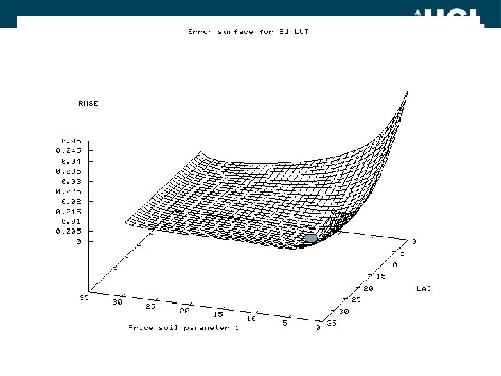
LUT Inversion • Sample parameter space • Calculate RMSE for each sample point • Define best fit as minimum RMSE parameters – Or function of set of points fitting to a certain tolerance • Essentially a sampled ‘exhaustive search’ http: //en. wikipedia. org/wiki/Lookup_table Gastellu et al. (2003) http: //ferrangascon. free. fr/publicacions/gastellu_gascon_esteve-2003 -RSE. pdf

LUT Inversion • Issues: – May require large sample set – Not so if function is well-behaved • In some cases, may assume function is locally linear over large (linearised) parameter range • Use linear interpolation – May limit search space based on some expectation • E. g. some loose relationship between observed system & parameters of interest • Eg for remote sensing canopy growth model or land cover map • Approach used for operational MODIS LAI/f. APAR algorithm (Myneni et al) • http: //modis. gsfc. nasa. gov/data/atbd_mod 15. pdf

LUT Inversion • Issues: – As operating on stored LUT, can pre-calculate model outputs • Don’t need to calculate model ‘on the fly’ as in e. g. simplex methods • Can use complex models to populate LUT – E. g. of Lewis, Saich & Disney using 3 D scattering models (optical and microwave) of forest and crop – Error in inversion may be slightly higher if (non-interpolated) sparse LUT • But may still lie within desirable limits – Method is simple to code and easy to understand • essentially a sort operation on a table http: //www 2. geog. ucl. ac. uk/~mdisney/igarss 03/FINAL/saich_lewis_disney. pdf

Summary: options for non-linear inversion • Gradient methods – Newton (1 st, 2 nd derivs. , ), Quasi-N (approx. 2 nd derivs eg BFGS) etc. • Non-gradient, ‘traditional’ methods: – Powell, AMOEBA • Complex to code – though library functions available • Can easily converge to local minima – Need to start at several points • Calculate canopy reflectance ‘on the fly’ – Need fast models, involving simplifications • Not felt to be suitable for operationalisation

Summary: options for non-linear inversion • Simulated Annealing – Slow & need to define annealing schedule – BUT can deal with local minima • ANNs – Train ANN from model (or measurements) to generalises as nonlinear model – Issues of variable input conditions – Can train with complex models • GAs – Novel approach, suitable for highly complex inversion problems – Can be very slow – Not suitable for operationalisation

Summary • LUT – Simple ‘brute force’ method • Sorting, few/no assumptions about model behaviour – Used more and more widely for operational model inversion • Suitable for ‘well-behaved’ non-linear problems – Can operationalise – Can use arbitrarily complex models to populate LUT – Issue of LUT size • Can use additional information to limit search space • Can use interpolation for sparse LUT for ‘high information content’ inversion