TRAFFIC FLOW MODELS USING SECONDORDER ORDINARY DIFFERENTIAL EQUATIONS

TRAFFIC FLOW MODELS USING SECOND-ORDER ORDINARY DIFFERENTIAL EQUATIONS Vane Petrosyan Mariam Balabanyan

Overview • What is traffic flow? • Mathematical model of traffic flow • Application of the model to investigate stopping distances – Solving an initial value problem using a linear, nonhomogenous, constant-coefficient, second-order differential equation

What is traffic flow and why is it important? Exploration of interactions between vehicles, drivers, and infrastructure in a general environment Goal of researchers: Generate a useful model Promote a road network with efficient movement of traffic and nominal traffic congestion interference Three variables: speed, flow and concentration

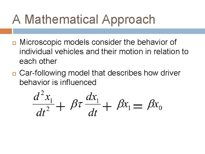
A Mathematical Approach Microscopic models consider the behavior of individual vehicles and their motion in relation to each other Car-following model that describes how driver behavior is influenced

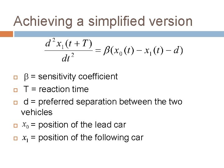
Achieving a simplified version b = sensitivity coefficient T = reaction time d = preferred separation between the two vehicles = position of the lead car = position of the following car

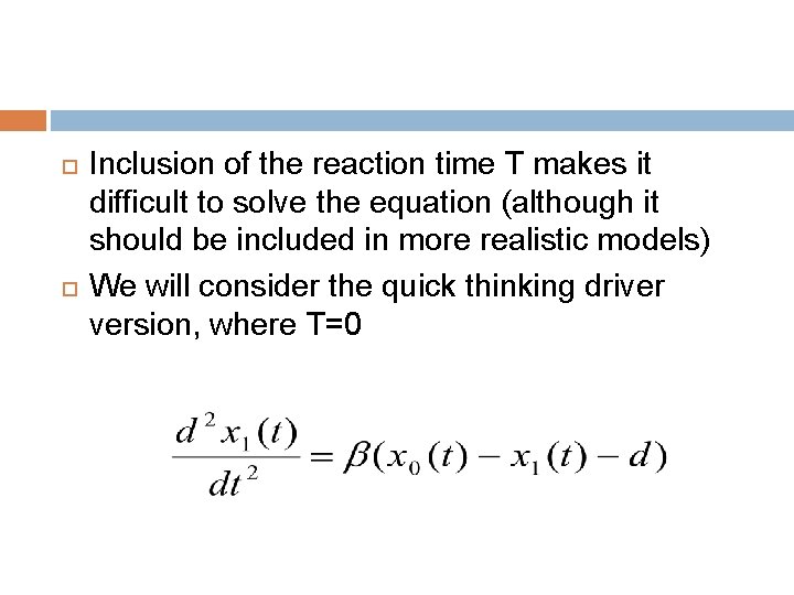
Inclusion of the reaction time T makes it difficult to solve the equation (although it should be included in more realistic models) We will consider the quick thinking driver version, where T=0

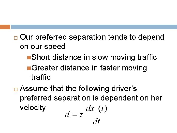
Our preferred separation tends to depend on our speed Short distance in slow moving traffic Greater distance in faster moving traffic Assume that the following driver’s preferred separation is dependent on her velocity

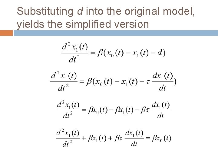
Substituting d into the original model, yields the simplified version

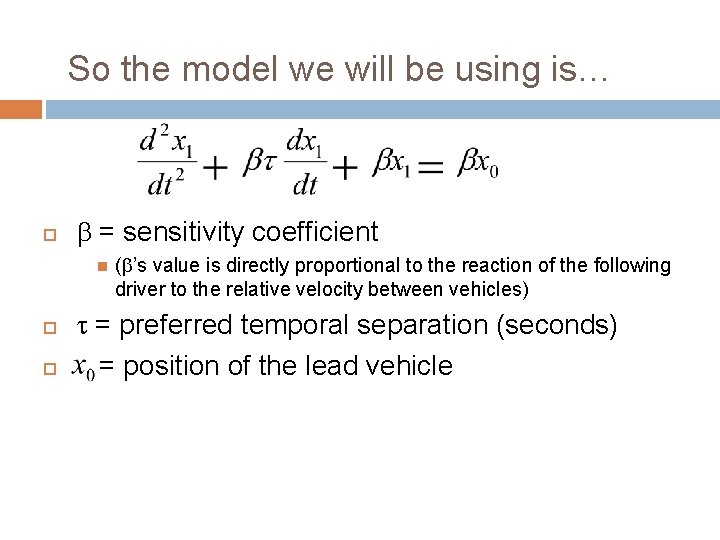
So the model we will be using is… b = sensitivity coefficient (b’s value is directly proportional to the reaction of the following driver to the relative velocity between vehicles) t = preferred temporal separation (seconds) = position of the lead vehicle

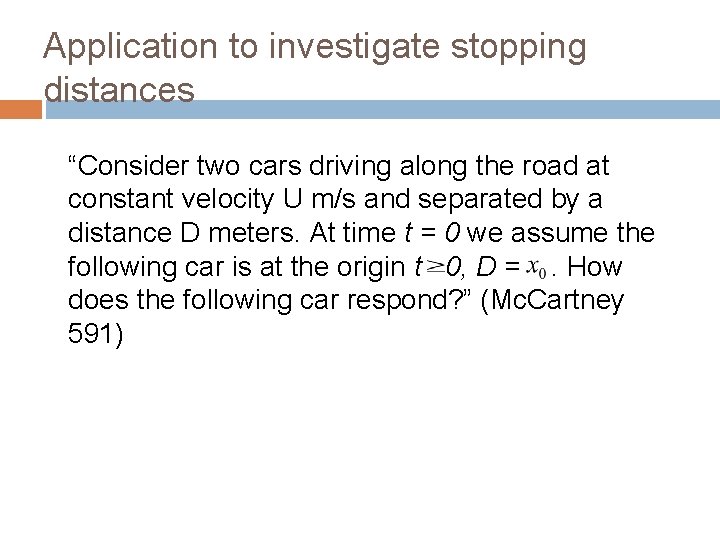
Application to investigate stopping distances “Consider two cars driving along the road at constant velocity U m/s and separated by a distance D meters. At time t = 0 we assume the following car is at the origin t 0, D =. How does the following car respond? ” (Mc. Cartney 591)

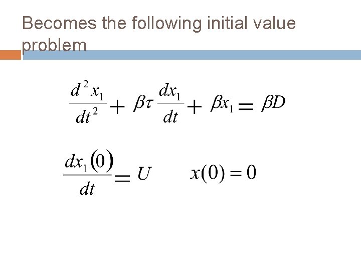
Becomes the following initial value problem

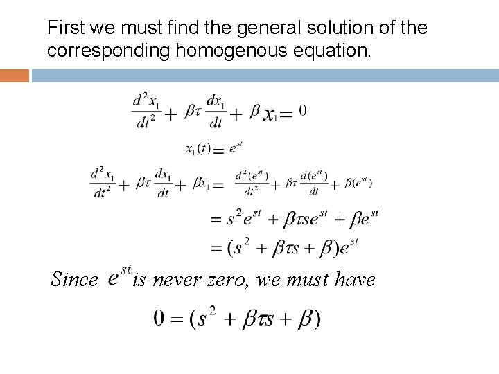
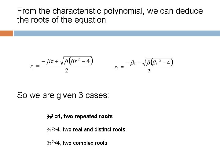
First we must find the general solution of the corresponding homogenous equation. Since is never zero, we must have

From the characteristic polynomial, we can deduce the roots of the equation So we are given 3 cases: bt 2 =4, two repeated roots bt 2>4, two real and distinct roots bt 2<4, two complex roots

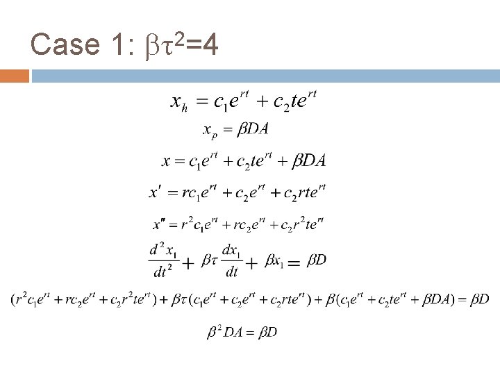
Case 1: bt 2=4

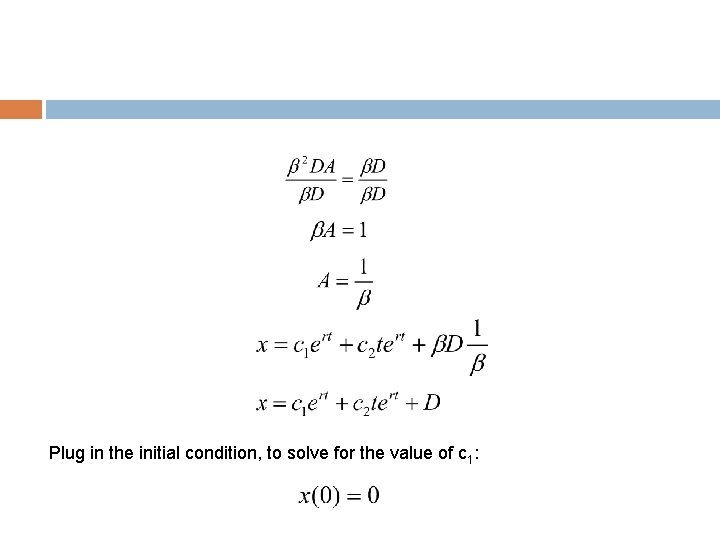
Plug in the initial condition, to solve for the value of c 1:

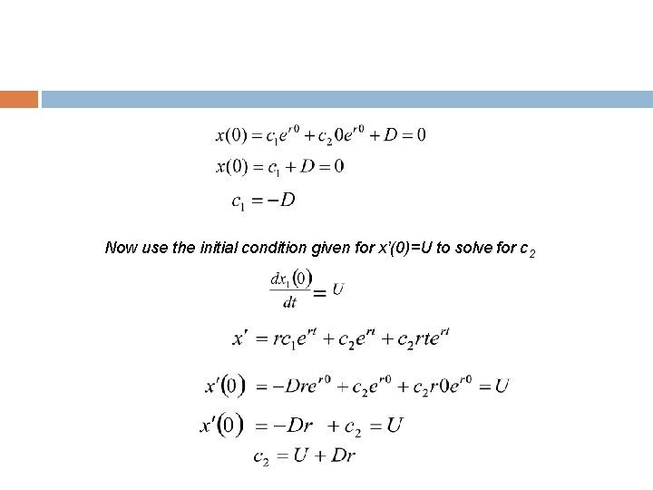
Now use the initial condition given for x’(0)=U to solve for c 2

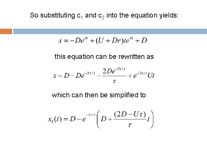
So substituting c 1 and c 2 into the equation yields: this equation can be rewritten as which can then be simplified to

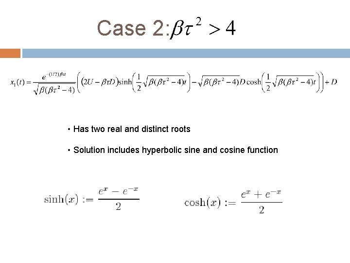
Case 2: • Has two real and distinct roots • Solution includes hyperbolic sine and cosine function

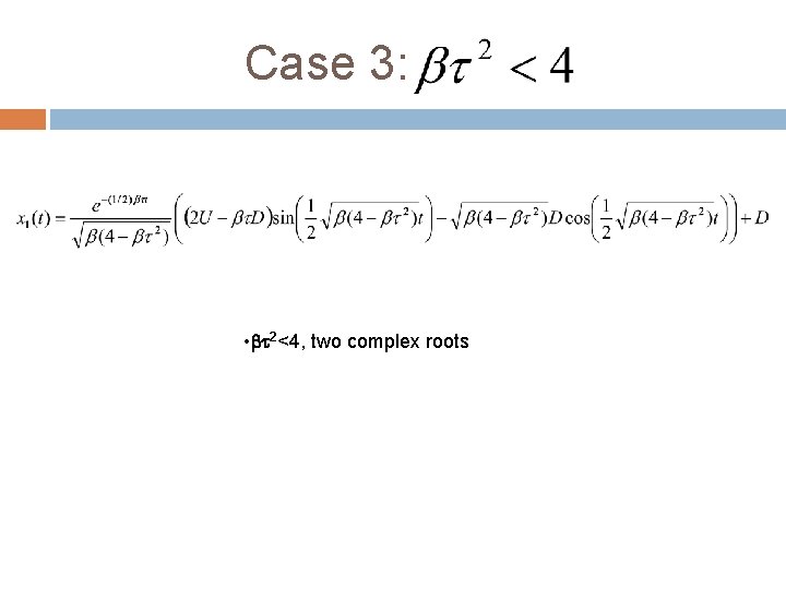
Case 3: • bt 2<4, two complex roots

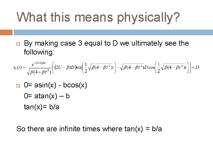
What this means physically? By making case 3 equal to D we ultimately see the following: 0= asin(x) - bcos(x) 0= atan(x) – b tan(x)= b/a So there are infinite times where tan(x) = b/a

Conclusion The mathematical model will only be physically meaningful if we restrict parameter values The driver may be quick thinking but the vehicle will infinitely collide the stopping distance is proportional to the initial velocity of the driver