Review of Macroeconomics THE ROOTS OF MACROECONOMICS THE

Review of Macroeconomics

THE ROOTS OF MACROECONOMICS THE GREAT DEPRESSION Great Depression The period of severe economic contraction and high unemployment that began in 1929 and continued throughout the 1930 s. 2 of 38

THE ROOTS OF MACROECONOMICS Classical Models Classical economists applied microeconomic models, or “market clearing” models, to economy-wide problems. Simple classical models failed to explain the prolonged existence of high unemployment during the Great Depression. This provided the impetus for the development of macroeconomics. 3 of 38

THE ROOTS OF MACROECONOMICS The Keynesian Revolution In 1936, John Maynard Keynes published The General Theory of Employment, Interest, and Money. Much of macroeconomics has roots in Keynes’s work. According to Keynes, it is not prices and wages that determine the level of employment, as classical models had suggested, but instead the level of aggregate demand for goods and services. 4 of 38

MACROECONOMIC CONCERNS Three of the major concerns of macroeconomics are: ■ Inflation ■ Output growth ■ Unemployment 5 of 38

MACROECONOMIC CONCERNS INFLATION AND DEFLATION inflation An increase in the overall price level. hyperinflation A period of very rapid increases in the overall price level. deflation A decrease in the overall price level. 6 of 38

MACROECONOMIC CONCERNS OUTPUT GROWTH: SHORT RUN AND LONG RUN business cycle The cycle of short-term ups and downs in the economy. aggregate output The total quantity of goods and services produced in an economy in a given period. 7 of 38

MACROECONOMIC CONCERNS recession A period during which aggregate output declines. Conventionally, a period in which aggregate output declines for two consecutive quarters. depression A prolonged and deep recession. 8 of 38

MACROECONOMIC CONCERNS UNEMPLOYMENT unemployment rate The percentage of the labor force that is unemployed. 9 of 38

GOVERNMENT IN THE MACROECONOMY There are three kinds of policy that the government has used to influence the macroeconomy: 1. Fiscal policy 2. Monetary policy 3. Growth or supply-side policies 10 of 38

GOVERNMENT IN THE MACROECONOMY FISCAL POLICY fiscal policy Government policies concerning taxes and expenditures (spending). 11 of 38

GOVERNMENT IN THE MACROECONOMY MONETARY POLICY monetary policy The tools used by the Federal Reserve to control the quantity of money in the economy. 12 of 38

GOVERNMENT IN THE MACROECONOMY GROWTH POLICIES supply-side policies Government policies that focus on stimulating aggregate supply instead of aggregate demand. 13 of 38

THE COMPONENTS OF THE MACROECONOMY Macroeconomics focuses on four groups: (1) households and (2) firms, which together compose the private sector, (3) the government (the public sector), and (4) the rest of the world (the international sector). 14 of 38

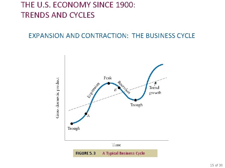
THE U. S. ECONOMY SINCE 1900: TRENDS AND CYCLES EXPANSION AND CONTRACTION: THE BUSINESS CYCLE FIGURE 5. 3 A Typical Business Cycle 15 of 38

THE U. S. ECONOMY SINCE 1900: TRENDS AND CYCLES expansion or boom The period in the business cycle from a trough up to a peak, during which output and employment rise. contraction, recession, or slump The period in the business cycle from a peak down to a trough, during which output and employment fall. 16 of 38

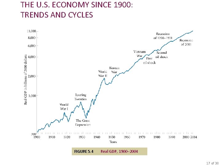
THE U. S. ECONOMY SINCE 1900: TRENDS AND CYCLES FIGURE 5. 4 Real GDP, 1900– 2004 17 of 38

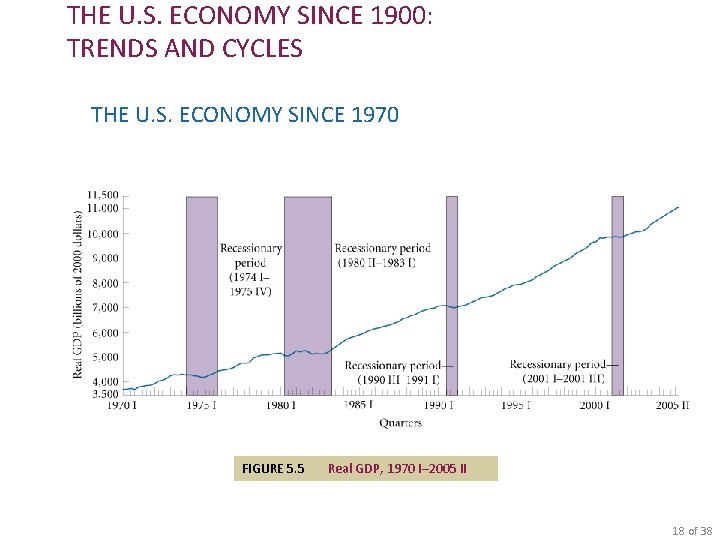
THE U. S. ECONOMY SINCE 1900: TRENDS AND CYCLES THE U. S. ECONOMY SINCE 1970 FIGURE 5. 5 Real GDP, 1970 I– 2005 II 18 of 38

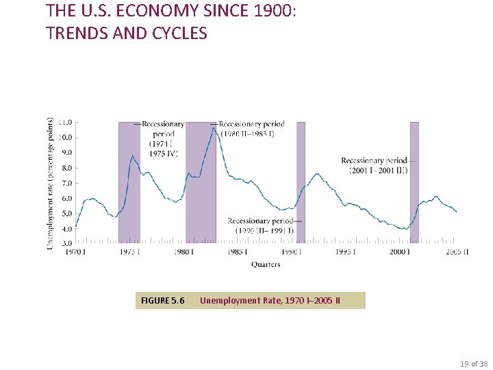
THE U. S. ECONOMY SINCE 1900: TRENDS AND CYCLES FIGURE 5. 6 Unemployment Rate, 1970 I– 2005 II 19 of 38

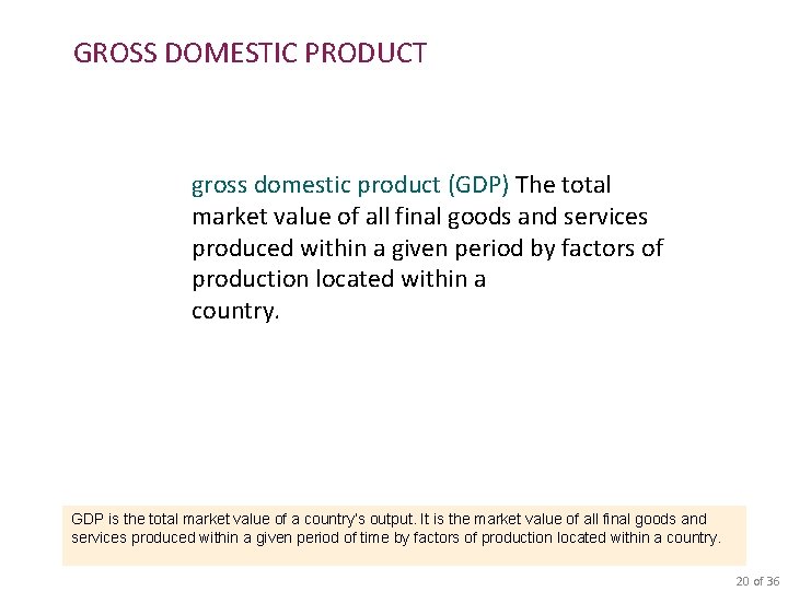
GROSS DOMESTIC PRODUCT gross domestic product (GDP) The total market value of all final goods and services produced within a given period by factors of production located within a country. GDP is the total market value of a country’s output. It is the market value of all final goods and services produced within a given period of time by factors of production located within a country. 20 of 36

GROSS DOMESTIC PRODUCT FINAL GOODS AND SERVICES final goods and services Goods and services produced for final use. intermediate goods Goods that are produced by one firm for use in further processing by another firm. value added The difference between the value of goods as they leave a stage of production and the cost of the goods as they entered that stage. 21 of 36

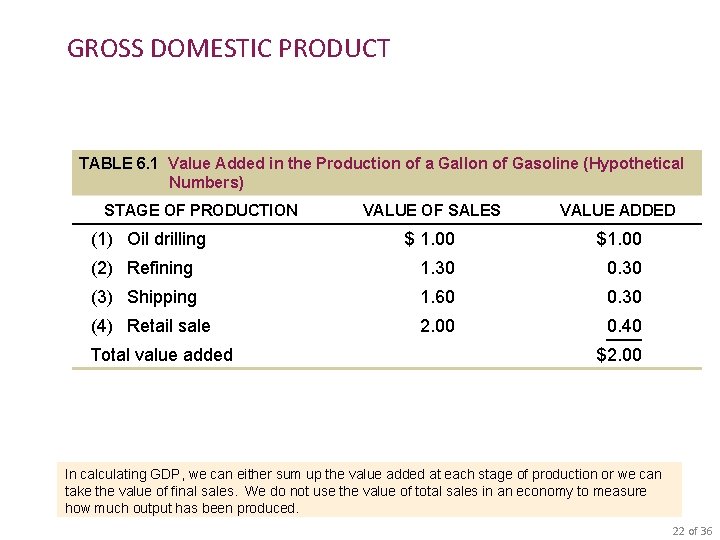
GROSS DOMESTIC PRODUCT TABLE 6. 1 Value Added in the Production of a Gallon of Gasoline (Hypothetical Numbers) STAGE OF PRODUCTION VALUE OF SALES VALUE ADDED $ 1. 00 $1. 00 (2) Refining 1. 30 0. 30 (3) Shipping 1. 60 0. 30 (4) Retail sale 2. 00 0. 40 (1) Oil drilling Total value added $2. 00 In calculating GDP, we can either sum up the value added at each stage of production or we can take the value of final sales. We do not use the value of total sales in an economy to measure how much output has been produced. 22 of 36

GROSS DOMESTIC PRODUCT EXCLUSION OF USED GOODS AND PAPER TRANSACTIONS GDP is concerned only with new, or current, production. GDP ignores all transactions in which money or goods change hands but in which no new goods and services are produced. 23 of 36

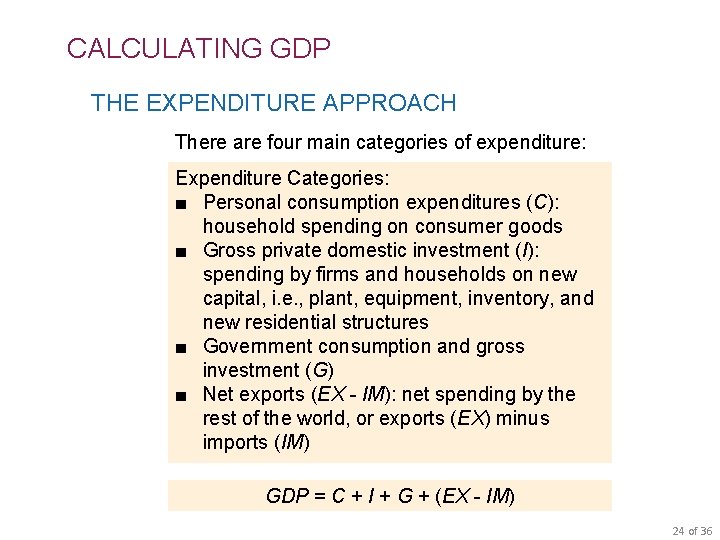
CALCULATING GDP THE EXPENDITURE APPROACH There are four main categories of expenditure: Expenditure Categories: ■ Personal consumption expenditures (C): household spending on consumer goods ■ Gross private domestic investment (I): spending by firms and households on new capital, i. e. , plant, equipment, inventory, and new residential structures ■ Government consumption and gross investment (G) ■ Net exports (EX - IM): net spending by the rest of the world, or exports (EX) minus imports (IM) GDP = C + I + G + (EX - IM) 24 of 36

CALCULATING GDP Personal Consumption Expenditures (C) personal consumption expenditures (C) A major component of GDP: expenditures by consumers on goods and services. There are three main categories of consumer expenditures: durable goods, nondurable goods, and services. 25 of 36

CALCULATING GDP durable goods Goods that last a relatively long time, such as cars and household appliances. nondurable goods Goods that are used up fairly quickly, such as food and clothing. services The things we buy that do not involve the production of physical things, such as legal and medical services and education. 26 of 36

CALCULATING GDP Gross Private Domestic Investment (I) gross private domestic investment (I) Total investment in capital—that is, the purchase of new housing, plants, equipment, and inventory by the private (or nongovernment) sector. nonresidential investment Expenditures by firms for machines, tools, plants, and so on. 27 of 36

CALCULATING GDP residential investment Expenditures by households and firms on new houses and apartment buildings. Change in Business Inventories change in business inventories The amount by which firms’ inventories change during a period. Inventories are the goods that firms produce now but intend to sell later. GDP = final sales + change in business inventories 28 of 36

CALCULATING GDP Gross Investment versus Net Investment depreciation The amount by which an asset’s value falls in a given period. gross investment The total value of all newly produced capital goods (plant, equipment, housing, and inventory) produced in a given period. net investment Gross investment minus depreciation. capitalend of period = capitalbeginning of period + net investment 29 of 36

CALCULATING GDP Government Consumption and Gross Investment (G) government consumption and gross investment (G) Expenditures by federal, state, and local governments for final goods and services. 30 of 36

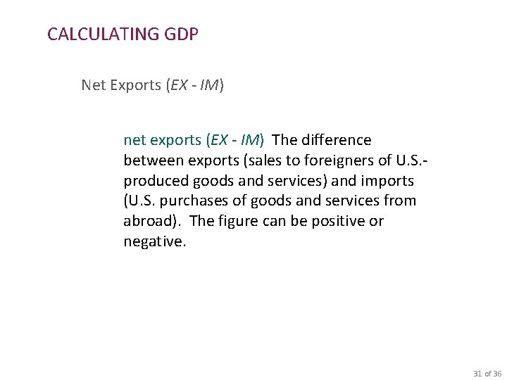
CALCULATING GDP Net Exports (EX - IM) net exports (EX - IM) The difference between exports (sales to foreigners of U. S. produced goods and services) and imports (U. S. purchases of goods and services from abroad). The figure can be positive or negative. 31 of 36

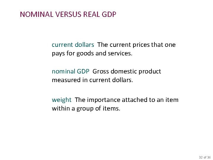
NOMINAL VERSUS REAL GDP current dollars The current prices that one pays for goods and services. nominal GDP Gross domestic product measured in current dollars. weight The importance attached to an item within a group of items. 32 of 36

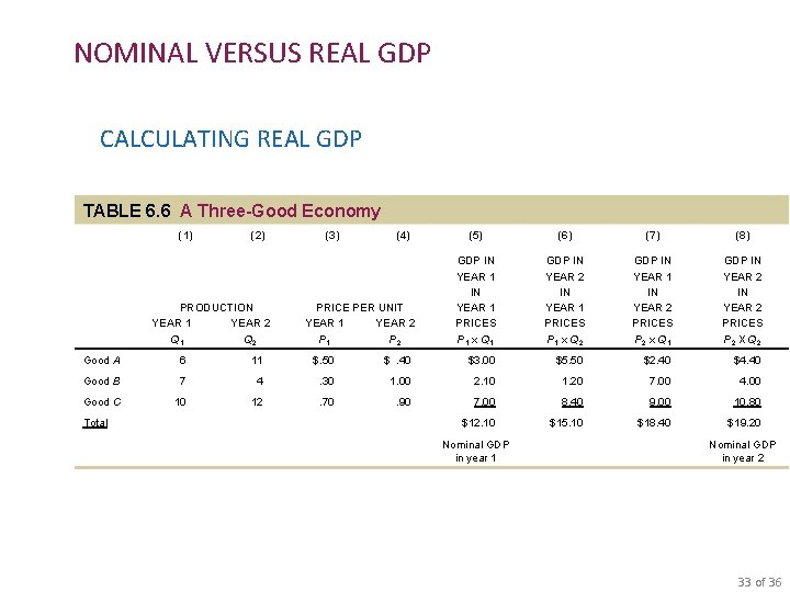
NOMINAL VERSUS REAL GDP CALCULATING REAL GDP TABLE 6. 6 A Three-Good Economy (1) (2) PRODUCTION YEAR 1 YEAR 2 Q 1 Q 2 (3) (4) PRICE PER UNIT YEAR 1 YEAR 2 P 1 P 2 (5) (6) (7) (8) GDP IN YEAR 1 PRICES P 1 x Q 1 GDP IN YEAR 2 IN YEAR 1 PRICES P 1 x Q 2 GDP IN YEAR 1 IN YEAR 2 PRICES P 2 x Q 1 GDP IN YEAR 2 PRICES P 2 X Q 2 Good A 6 11 $. 50 $. 40 $3. 00 $5. 50 $2. 40 $4. 40 Good B 7 4 . 30 1. 00 2. 10 1. 20 7. 00 4. 00 Good C 10 12 . 70 . 90 7. 00 8. 40 9. 00 10. 80 $12. 10 $15. 10 $18. 40 $19. 20 Total Nominal GDP in year 1 Nominal GDP in year 2 33 of 36

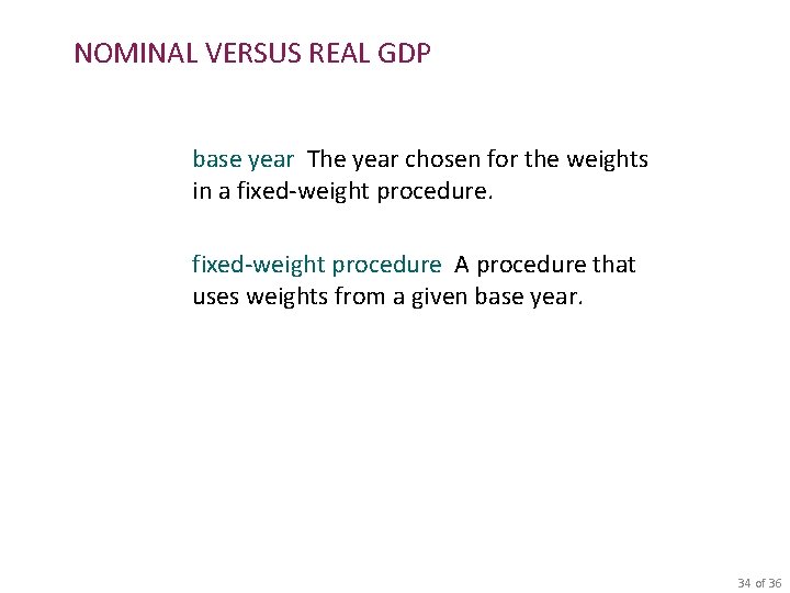
NOMINAL VERSUS REAL GDP base year The year chosen for the weights in a fixed-weight procedure A procedure that uses weights from a given base year. 34 of 36

NOMINAL VERSUS REAL GDP CALCULATING THE GDP DEFLATOR The GDP deflator is one measure of the overall price level. The GDP deflator is computed by the Bureau of Economic Analysis (BEA). Overall price increases can be sensitive to the choice of the base year. For this reason, using fixed-price weights to compute real GDP has some problems. 35 of 36

NOMINAL VERSUS REAL GDP THE PROBLEMS OF FIXED WEIGHTS The use of fixed-price weights to estimate real GDP leads to problems because it ignores: • Structural changes in the economy. • Supply shifts, which cause large decreases in price and large increases in quantity supplied. • The substitution effect of price increases. 36 of 36

LIMITATIONS OF THE GDP CONCEPT GDP AND SOCIAL WELFARE Society is better off when crime decreases; however, a decrease in crime is not reflected in GDP. An increase in leisure is an increase in social welfare, but not counted in GDP. Nonmarket and household activities are not counted in GDP even though they amount to real production. 37 of 36

Unemployment Measuring Unemployment employed Any person 16 years old or older (1) who works for pay, either for someone else or in his or her own business for 1 or more hours per week, (2) who works without pay for 15 or more hours per week in a family enterprise, or (3) who has a job but has been temporarily absent with or without pay. unemployed A person 16 years old or older who is not working, is available for work, and has made specific efforts to find work during the previous 4 weeks. 38 of 25

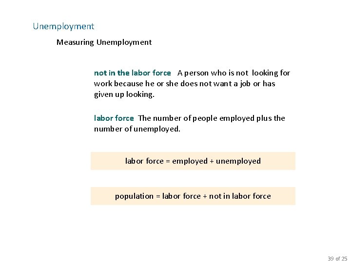
Unemployment Measuring Unemployment not in the labor force A person who is not looking for work because he or she does not want a job or has given up looking. labor force The number of people employed plus the number of unemployed. labor force = employed + unemployed population = labor force + not in labor force 39 of 25

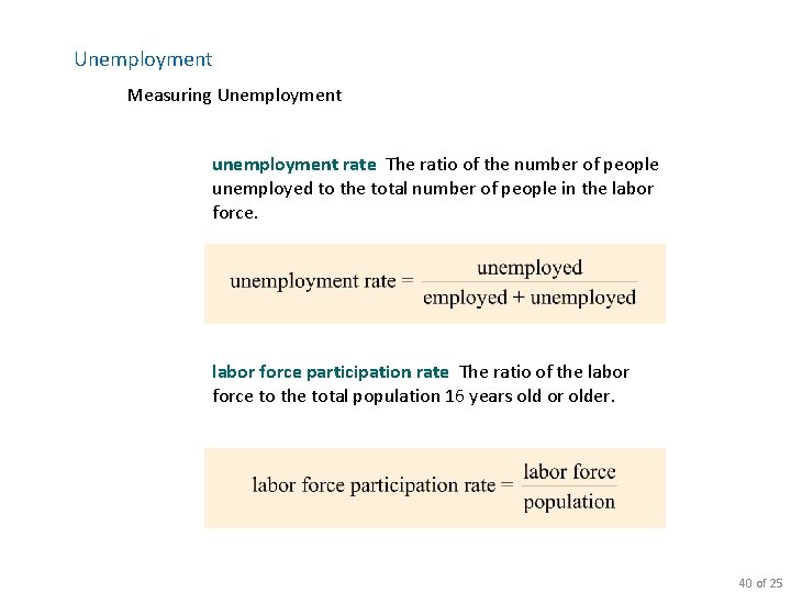
Unemployment Measuring Unemployment unemployment rate The ratio of the number of people unemployed to the total number of people in the labor force participation rate The ratio of the labor force to the total population 16 years old or older. 40 of 25

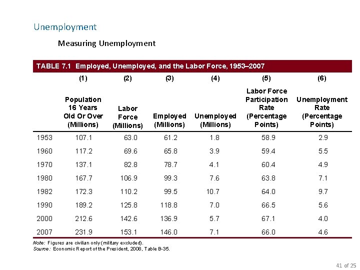
Unemployment Measuring Unemployment TABLE 7. 1 Employed, Unemployed, and the Labor Force, 1953– 2007 (1) Population 16 Years Old Or Over (Millions) (2) Labor Force (Millions) (3) (4) (5) (6) Employed (Millions) Unemployed (Millions) Labor Force Participation Rate (Percentage Points) Unemployment Rate (Percentage Points) 1953 107. 1 63. 0 61. 2 1. 8 58. 9 2. 9 1960 117. 2 69. 6 65. 8 3. 9 59. 4 5. 5 1970 137. 1 82. 8 78. 7 4. 1 60. 4 4. 9 1980 167. 7 106. 9 99. 3 7. 6 63. 8 7. 1 1982 172. 3 110. 2 99. 5 10. 7 64. 0 9. 7 1990 189. 2 125. 8 118. 8 7. 0 66. 5 5. 6 2000 212. 6 142. 6 136. 9 5. 7 67. 1 4. 0 2007 231. 9 153. 1 146. 0 7. 1 66. 0 4. 6 Note: Figures are civilian only (military excluded). Source: Economic Report of the President, 2008, Table B-35. 41 of 25

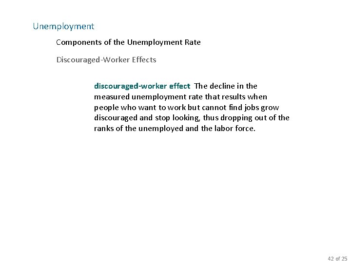
Unemployment Components of the Unemployment Rate Discouraged-Worker Effects discouraged-worker effect The decline in the measured unemployment rate that results when people who want to work but cannot find jobs grow discouraged and stop looking, thus dropping out of the ranks of the unemployed and the labor force. 42 of 25

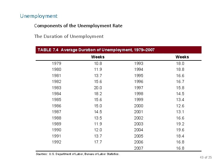
Unemployment Components of the Unemployment Rate The Duration of Unemployment TABLE 7. 4 Average Duration of Unemployment, 1979– 2007 Weeks 1979 1980 1981 1982 1983 1984 1985 1986 1987 1988 1989 1990 1991 1992 10. 8 11. 9 13. 7 15. 6 20. 0 18. 2 15. 6 15. 0 14. 5 13. 5 11. 9 12. 0 13. 7 17. 7 Sources: U. S. Department of Labor, Bureau of Labor Statistics. Weeks 1993 1994 1995 1996 1997 1998 1999 2000 2001 2002 2003 2004 2005 2006 2007 18. 0 18. 8 16. 6 16. 7 15. 8 14. 5 13. 4 12. 6 13. 1 16. 6 19. 2 19. 6 18. 4 16. 8 43 of 25

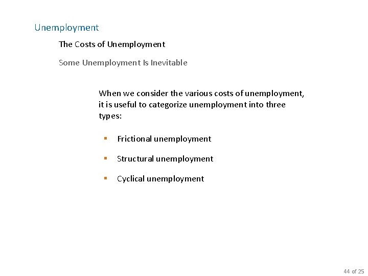
Unemployment The Costs of Unemployment Some Unemployment Is Inevitable When we consider the various costs of unemployment, it is useful to categorize unemployment into three types: § Frictional unemployment § Structural unemployment § Cyclical unemployment 44 of 25

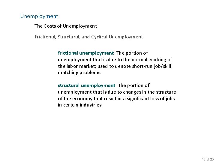
Unemployment The Costs of Unemployment Frictional, Structural, and Cyclical Unemployment frictional unemployment The portion of unemployment that is due to the normal working of the labor market; used to denote short-run job/skill matching problems. structural unemployment The portion of unemployment that is due to changes in the structure of the economy that result in a significant loss of jobs in certain industries. 45 of 25

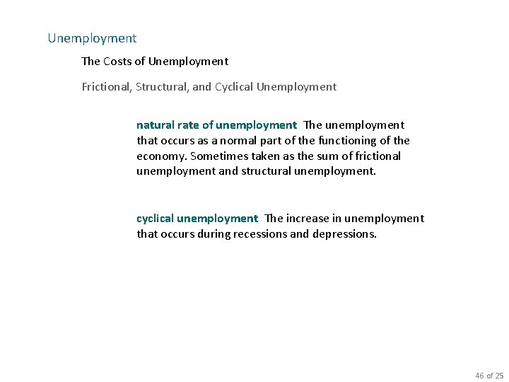
Unemployment The Costs of Unemployment Frictional, Structural, and Cyclical Unemployment natural rate of unemployment The unemployment that occurs as a normal part of the functioning of the economy. Sometimes taken as the sum of frictional unemployment and structural unemployment. cyclical unemployment The increase in unemployment that occurs during recessions and depressions. 46 of 25

Unemployment The Costs of Unemployment Social Consequences In addition to economic hardship, prolonged unemployment may also bring with it social and personal ills: anxiety, depression, deterioration of physical and psychological health, drug abuse (including alcoholism), and suicide. 47 of 25

THE CONSUMER PRICE INDEX The consumer price index (CPI) is a measure of the overall cost of the goods and services bought by a typical consumer. The Bureau of Labor Statistics reports the CPI each month. It is used to monitor changes in the cost of living over time.

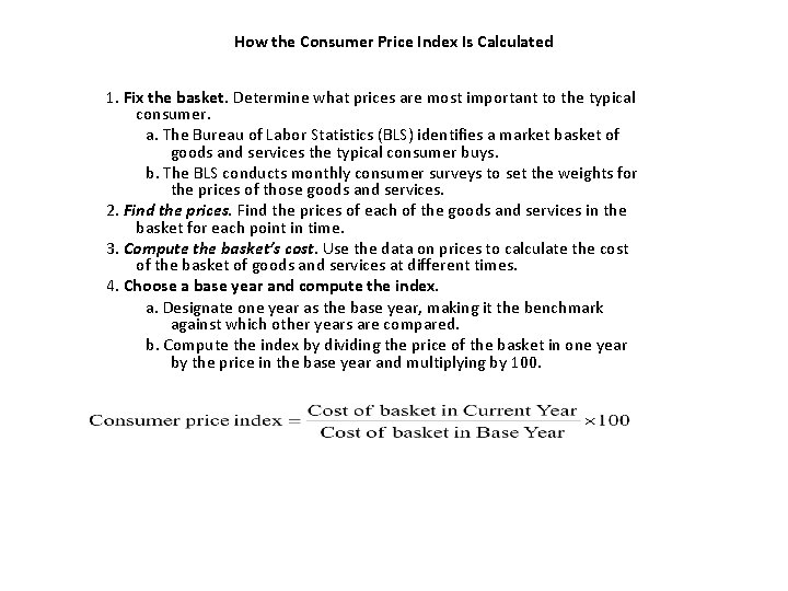
How the Consumer Price Index Is Calculated 1. Fix the basket. Determine what prices are most important to the typical consumer. a. The Bureau of Labor Statistics (BLS) identifies a market basket of goods and services the typical consumer buys. b. The BLS conducts monthly consumer surveys to set the weights for the prices of those goods and services. 2. Find the prices of each of the goods and services in the basket for each point in time. 3. Compute the basket’s cost. Use the data on prices to calculate the cost of the basket of goods and services at different times. 4. Choose a base year and compute the index. a. Designate one year as the base year, making it the benchmark against which other years are compared. b. Compute the index by dividing the price of the basket in one year by the price in the base year and multiplying by 100.

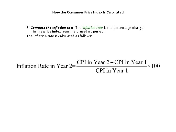
How the Consumer Price Index Is Calculated 5. Compute the inflation rate. The inflation rate is the percentage change in the price index from the preceding period. The inflation rate is calculated as follows:

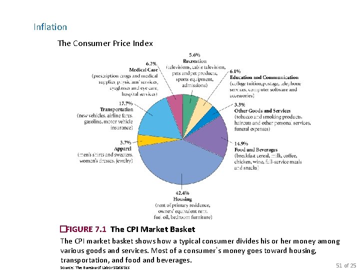
Inflation The Consumer Price Index �FIGURE 7. 1 The CPI Market Basket The CPI market basket shows how a typical consumer divides his or her money among various goods and services. Most of a consumer’s money goes toward housing, transportation, and food and beverages. Source: The Bureau of Labor Statistics 51 of 25

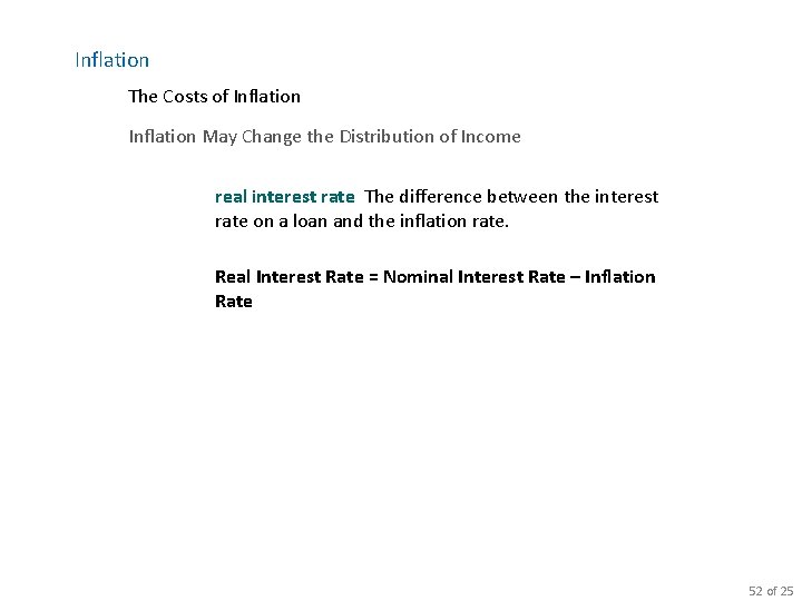
Inflation The Costs of Inflation May Change the Distribution of Income real interest rate The difference between the interest rate on a loan and the inflation rate. Real Interest Rate = Nominal Interest Rate – Inflation Rate 52 of 25

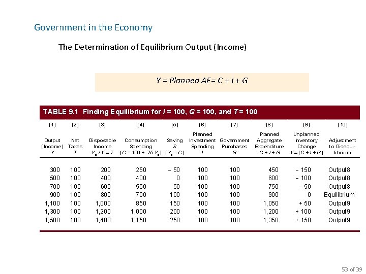
Government in the Economy The Determination of Equilibrium Output (Income) Y = Planned AE= C + I + G TABLE 9. 1 Finding Equilibrium for I = 100, G = 100, and T = 100 (1) (2) Output (Income) Y Net Taxes T 300 500 700 900 1, 100 1, 300 1, 500 100 100 (3) (4) (5) Disposable Consumption Saving Income Spending S Yd / Y T (C = 100 +. 75 Yd) (Yd – C) 200 400 600 800 1, 000 1, 200 1, 400 250 400 550 700 850 1, 000 1, 150 - 50 0 50 100 150 200 250 (6) (7) Planned Investment Government Spending Purchases I G 100 100 100 100 (8) (9) (10) Planned Aggregate Expenditure C+I+G Unplanned Inventory Change Y (C + I + G) Adjustment to Disequilibrium 450 600 750 900 1, 050 1, 200 1, 350 - 100 - 50 0 + 50 + 100 + 150 Output 8 Equilibrium Output 9 53 of 39

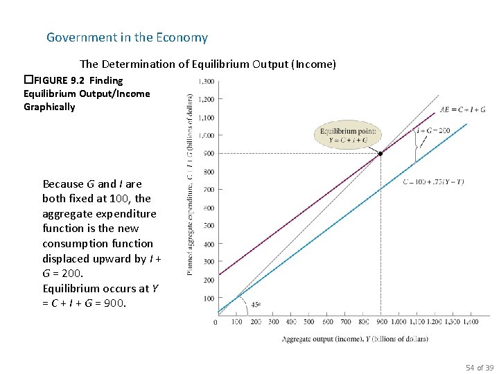
Government in the Economy The Determination of Equilibrium Output (Income) �FIGURE 9. 2 Finding Equilibrium Output/Income Graphically Because G and I are both fixed at 100, the aggregate expenditure function is the new consumption function displaced upward by I + G = 200. Equilibrium occurs at Y = C + I + G = 900. 54 of 39

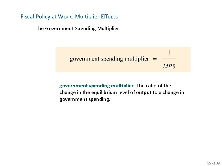
Fiscal Policy at Work: Multiplier Effects The Government Spending Multiplier government spending multiplier The ratio of the change in the equilibrium level of output to a change in government spending. 55 of 39

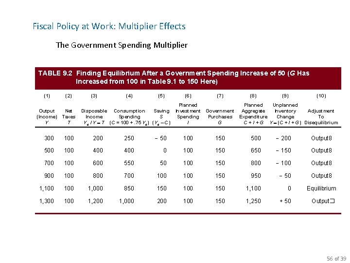
Fiscal Policy at Work: Multiplier Effects The Government Spending Multiplier TABLE 9. 2 Finding Equilibrium After a Government Spending Increase of 50 (G Has Increased from 100 in Table 9. 1 to 150 Here) (1) (2) Output (Income) Y Net Taxes T (3) (4) (5) Disposable Consumption Saving Income Spending S Yd / Y T (C = 100 +. 75 Yd) (Yd – C) (6) (7) Planned Investment Government Spending Purchases I G (8) (9) (10) Planned Unplanned Aggregate Inventory Adjustment Expenditure Change To C + I + G Y (C + I + G) Disequilibrium 300 100 250 - 50 100 150 500 - 200 Output 8 500 100 400 0 100 150 650 - 150 Output 8 700 100 600 550 50 100 150 800 - 100 Output 8 900 100 800 700 100 150 950 - 50 Output 8 1, 100 1, 000 850 100 150 1, 100 0 Equilibrium 1, 300 1, 200 1, 000 200 150 1, 250 + 50 Output� 56 of 39

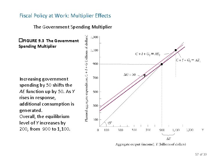
Fiscal Policy at Work: Multiplier Effects The Government Spending Multiplier �FIGURE 9. 3 The Government Spending Multiplier Increasing government spending by 50 shifts the AE function up by 50. As Y rises in response, additional consumption is generated. Overall, the equilibrium level of Y increases by 200, from 900 to 1, 100. 57 of 39

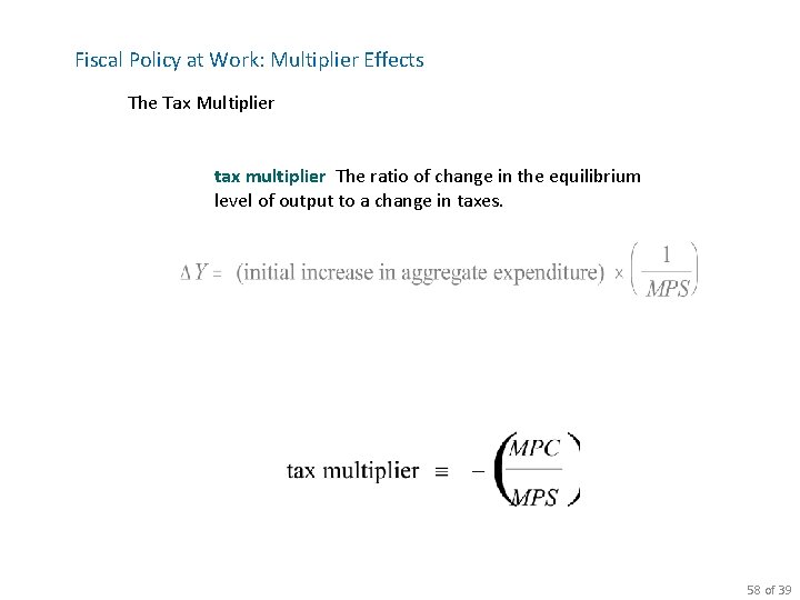
Fiscal Policy at Work: Multiplier Effects The Tax Multiplier tax multiplier The ratio of change in the equilibrium level of output to a change in taxes. 58 of 39

The Federal Budget federal budget The budget of the federal government. The “budget” is really three different budgets. First, it is a political document that dispenses favors to certain groups or regions and places burdens on others. Second, it is a reflection of goals the government wants to achieve. Third, the budget may be an embodiment of some beliefs about how (if at all) the government should manage the macroeconomy. 59 of 39

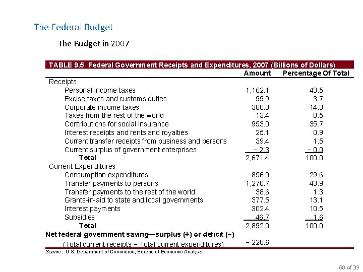
The Federal Budget The Budget in 2007 TABLE 9. 5 Federal Government Receipts and Expenditures, 2007 (Billions of Dollars) Amount Percentage Of Total Receipts Personal income taxes 1, 162. 1 43. 5 Excise taxes and customs duties 99. 9 3. 7 Corporate income taxes 380. 8 14. 3 Taxes from the rest of the world 13. 4 0. 5 Contributions for social insurance 953. 0 35. 7 Interest receipts and rents and royalties 25. 1 0. 9 Current transfer receipts from business and persons 39. 4 1. 5 Current surplus of government enterprises − 2. 3 − 0. 0 Total 2, 671. 4 100. 0 Current Expenditures Consumption expenditures 856. 0 29. 6 Transfer payments to persons 1, 270. 7 43. 9 Transfer payments to the rest of the world 38. 6 1. 3 Grants-in-aid to state and local governments 377. 5 13. 1 Interest payments 302. 4 10. 5 Subsidies 46. 7 1. 6 Total 2, 892. 0 100. 0 Net federal government saving—surplus (+) or deficit (−) − 220. 6 (Total current receipts − Total current expenditures) Source: U. S. Department of Commerce, Bureau of Economic Analysis. 60 of 39

The Federal Budget The Budget in 2007 federal surplus (+) or deficit ( ) Federal government receipts minus expenditures. 61 of 39

The Federal Budget The Federal Government Debt federal debt The total amount owed by the federal government. privately held federal debt The privately held (non-government-owned) debt of the U. S. government. 62 of 39

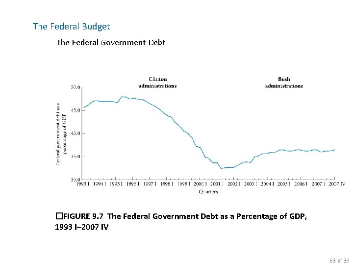
The Federal Budget The Federal Government Debt �FIGURE 9. 7 The Federal Government Debt as a Percentage of GDP, 1993 I– 2007 IV 63 of 39

The Economy’s Influence on the Government Budget Tax Revenues Depend on the State of the Economy Tax revenue, on the other hand, depends on taxable income, and income depends on the state of the economy, which the government does not completely control. Some Government Expenditures Depend on the State of the Economy Transfer payments tend to go down automatically during an expansion. Inflation often picks up when the economy is expanding. This can lead the government to spend more than it had planned to spend. Any change in the interest rate changes government interest payments. 64 of 39

The Economy’s Influence on the Government Budget Automatic Stabilizers automatic stabilizers Revenue and expenditure items in the federal budget that automatically change with the state of the economy in such a way as to stabilize GDP. Automatic De-Stabilizers: Any Thoughts? Fiscal Drag fiscal drag The negative effect on the economy that occurs when average tax rates increase because taxpayers have moved into higher income brackets during an expansion. 65 of 39

An Overview of Money What Is Money? A Store of Value store of value An asset that can be used to transport purchasing power from one time period to another. liquidity property of money The property of money that makes it a good medium of exchange as well as a store of value: It is portable and readily accepted and thus easily exchanged for goods. A Unit of Account unit of account A standard unit that provides a consistent way of quoting prices. 66 of 31

An Overview of Money Commodity and Fiat Monies commodity monies Items used as money that also have intrinsic value in some other use. fiat, or token, money Items designated as money that are intrinsically worthless. legal tender Money that a government has required to be accepted in settlement of debts. currency debasement The decrease in the value of money that occurs when its supply is increased rapidly. 67 of 31

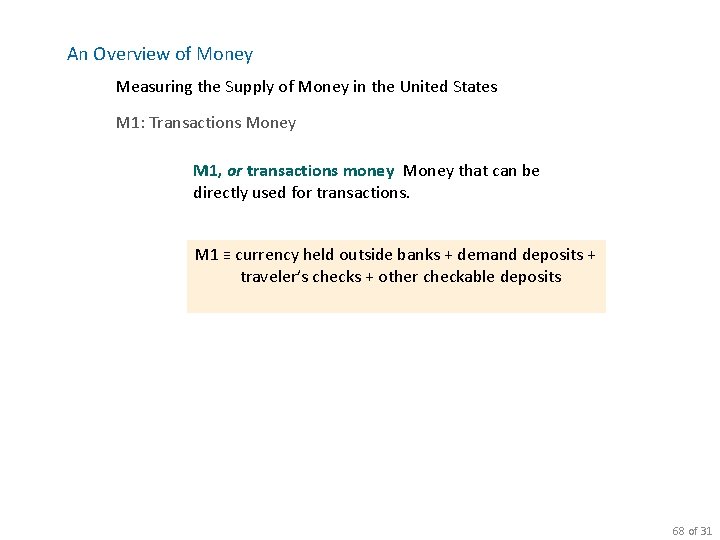
An Overview of Money Measuring the Supply of Money in the United States M 1: Transactions Money M 1, or transactions money Money that can be directly used for transactions. M 1 ≡ currency held outside banks + demand deposits + traveler’s checks + other checkable deposits 68 of 31

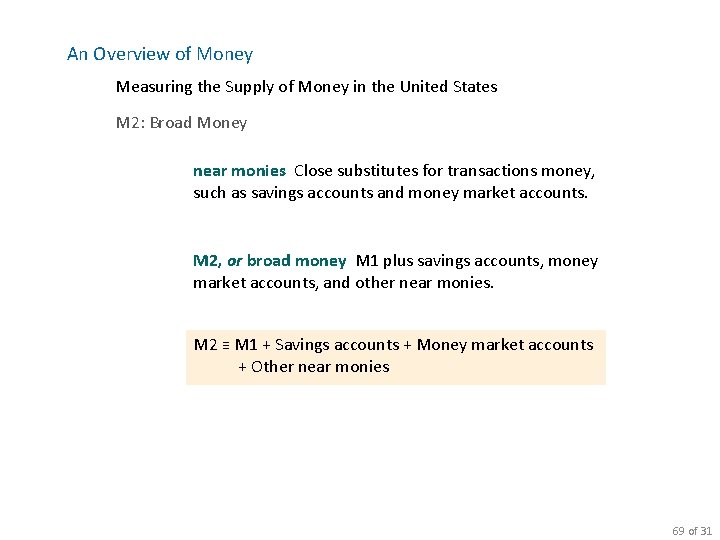
An Overview of Money Measuring the Supply of Money in the United States M 2: Broad Money near monies Close substitutes for transactions money, such as savings accounts and money market accounts. M 2, or broad money M 1 plus savings accounts, money market accounts, and other near monies. M 2 ≡ M 1 + Savings accounts + Money market accounts + Other near monies 69 of 31

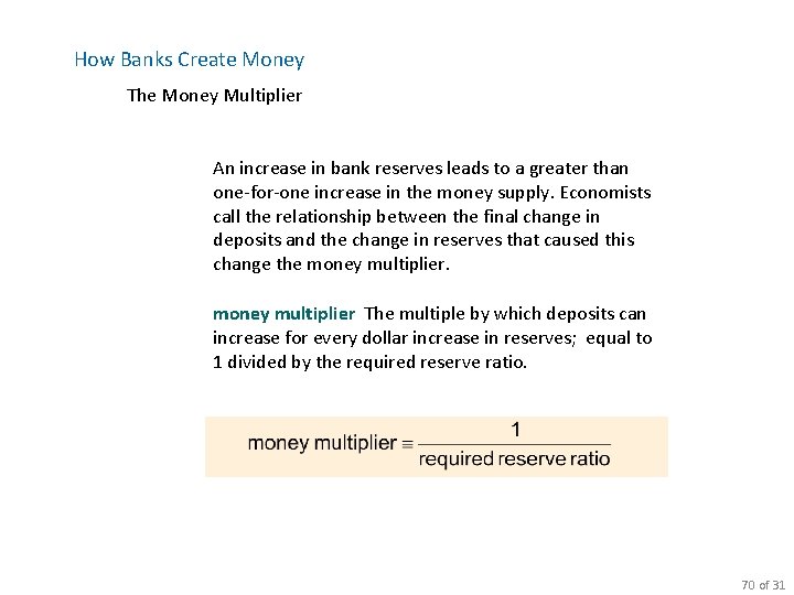
How Banks Create Money The Money Multiplier An increase in bank reserves leads to a greater than one-for-one increase in the money supply. Economists call the relationship between the final change in deposits and the change in reserves that caused this change the money multiplier The multiple by which deposits can increase for every dollar increase in reserves; equal to 1 divided by the required reserve ratio. 70 of 31

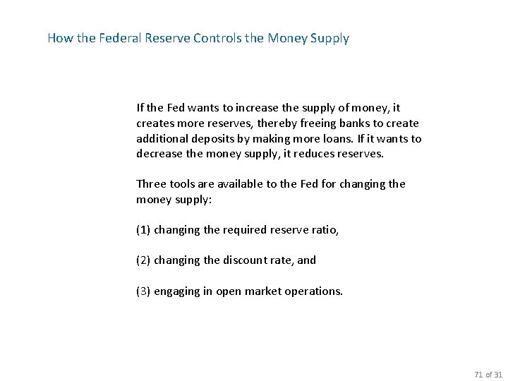
How the Federal Reserve Controls the Money Supply If the Fed wants to increase the supply of money, it creates more reserves, thereby freeing banks to create additional deposits by making more loans. If it wants to decrease the money supply, it reduces reserves. Three tools are available to the Fed for changing the money supply: (1) changing the required reserve ratio, (2) changing the discount rate, and (3) engaging in open market operations. 71 of 31

How the Federal Reserve Controls the Money Supply The Required Reserve Ratio Decreases in the required reserve ratio allow banks to have more deposits with the existing volume of reserves. As banks create more deposits by making loans, the supply of money (currency + deposits) increases. The reverse is also true: If the Fed wants to restrict the supply of money, it can raise the required reserve ratio, in which case banks will find that they have insufficient reserves and must therefore reduce their deposits by “calling in” some of their loans. The result is a decrease in the money supply. 72 of 31

How the Federal Reserve Controls the Money Supply The Discount Rate discount rate The interest rate that banks pay to the Fed to borrow from it. moral suasion The pressure that in the past the Fed exerted on member banks to discourage them from borrowing heavily from the Fed. 73 of 31

How the Federal Reserve Controls the Money Supply Open Market Operations open market operations The purchase and sale by the Fed of government securities in the open market; a tool used to expand or contract the amount of reserves in the system and thus the money supply. 74 of 31

How the Federal Reserve Controls the Money Supply Open Market Operations Two Branches of Government Deal in Government Securities The Treasury Department is responsible for collecting taxes and paying the federal government’s bills. The Fed is not the Treasury. Instead, it is a quasiindependent agency authorized by Congress to buy and sell outstanding (preexisting) U. S. government securities on the open market. 75 of 31

The Demand for Money When we speak of the demand for money, we are concerned with how much of your financial assets you want to hold in the form of money, which does not earn interest, versus how much you want to hold in interest-bearing securities, such as bonds. The Transaction Motive transaction motive The main reason that people hold money—to buy things. 76 of 23

The Demand for Money The Transaction Motive nonsynchronization of income and spending The mismatch between the timing of money inflow to the household and the timing of money outflow for household expenses. 77 of 23

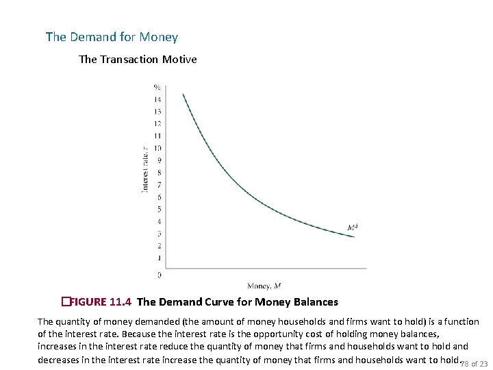
The Demand for Money The Transaction Motive �FIGURE 11. 4 The Demand Curve for Money Balances The quantity of money demanded (the amount of money households and firms want to hold) is a function of the interest rate. Because the interest rate is the opportunity cost of holding money balances, increases in the interest rate reduce the quantity of money that firms and households want to hold and decreases in the interest rate increase the quantity of money that firms and households want to hold. 78 of 23

The Demand for Money The Speculation Motive speculation motive One reason for holding bonds instead of money: Because the market price of interest -bearing bonds is inversely related to the interest rate, investors may want to hold bonds when interest rates are high with the hope of selling them when interest rates fall. 79 of 23

The Demand for Money The Total Demand for Money The total quantity of money demanded in the economy is the sum of the demand for checking account balances and cash by both households and firms. At any given moment, there is a demand for money— for cash and checking account balances. Although households and firms need to hold balances for everyday transactions, their demand has a limit. For both households and firms, the quantity of money demanded at any moment depends on the opportunity cost of holding money, a cost determined by the interest rate. 80 of 23

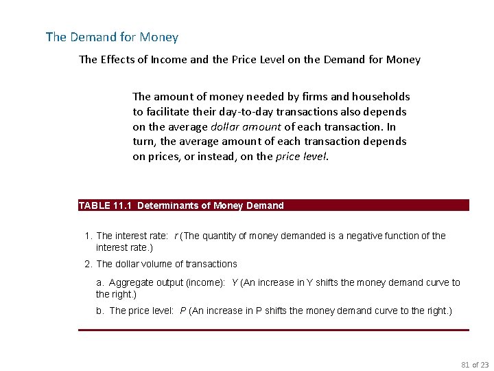
The Demand for Money The Effects of Income and the Price Level on the Demand for Money The amount of money needed by firms and households to facilitate their day-to-day transactions also depends on the average dollar amount of each transaction. In turn, the average amount of each transaction depends on prices, or instead, on the price level. TABLE 11. 1 Determinants of Money Demand 1. The interest rate: r (The quantity of money demanded is a negative function of the interest rate. ) 2. The dollar volume of transactions a. Aggregate output (income): Y (An increase in Y shifts the money demand curve to the right. ) b. The price level: P (An increase in P shifts the money demand curve to the right. ) 81 of 23

The Equilibrium Interest Rate We are now in a position to consider one of the key questions in macroeconomics : How is the interest rate determined in the economy? The point at which the quantity of money demanded equals the quantity of money supplied determines the equilibrium interest rate in the economy. 82 of 23

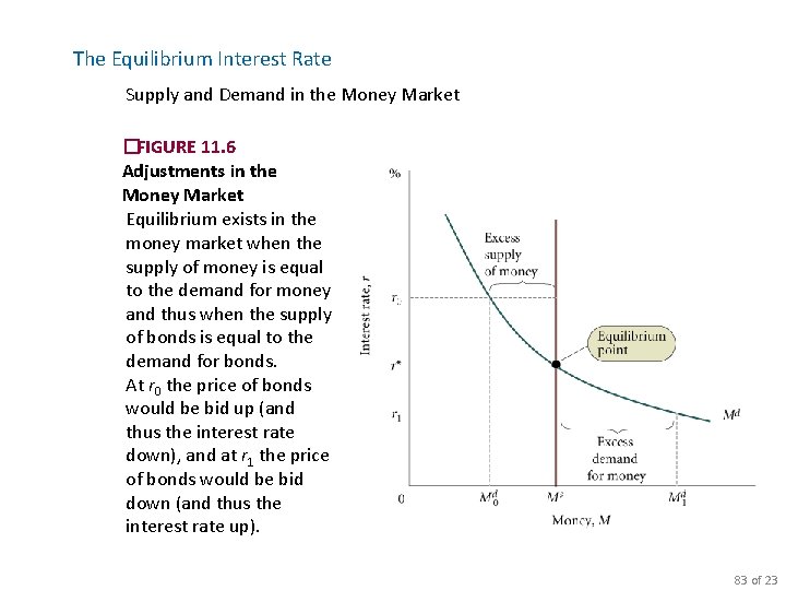
The Equilibrium Interest Rate Supply and Demand in the Money Market �FIGURE 11. 6 Adjustments in the Money Market Equilibrium exists in the money market when the supply of money is equal to the demand for money and thus when the supply of bonds is equal to the demand for bonds. At r 0 the price of bonds would be bid up (and thus the interest rate down), and at r 1 the price of bonds would be bid down (and thus the interest rate up). 83 of 23

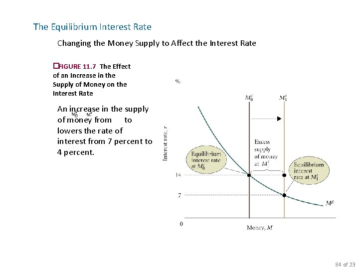
The Equilibrium Interest Rate Changing the Money Supply to Affect the Interest Rate �FIGURE 11. 7 The Effect of an Increase in the Supply of Money on the Interest Rate An increase in the supply of money from to lowers the rate of interest from 7 percent to 4 percent. 84 of 23

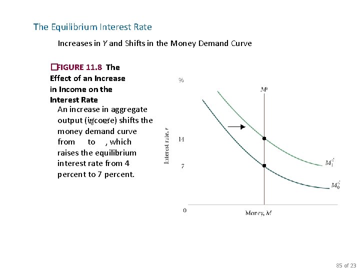
The Equilibrium Interest Rate Increases in Y and Shifts in the Money Demand Curve �FIGURE 11. 8 The Effect of an Increase in Income on the Interest Rate An increase in aggregate output (income) shifts the money demand curve from to , which raises the equilibrium interest rate from 4 percent to 7 percent. 85 of 23

Looking Ahead: The Federal Reserve and Monetary Policy tight monetary policy Fed policies that contract the money supply and thus raise interest rates in an effort to restrain the economy. easy monetary policy Fed policies that expand the money supply and thus lower interest rates in an effort to stimulate the economy. 86 of 23

Aggregate Demand in the Goods and Money Markets goods market The market in which goods and services are exchanged and in which the equilibrium level of aggregate output is determined. money market The market in which financial instruments are exchanged and in which the equilibrium level of the interest rate is determined. 87 of 37

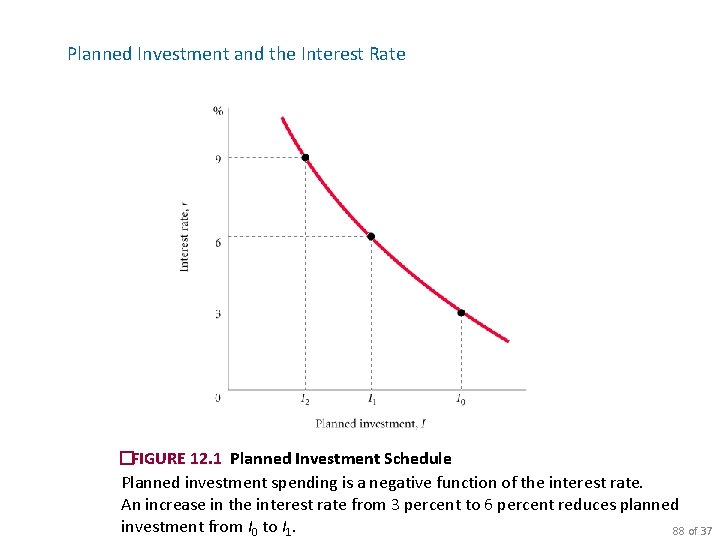
Planned Investment and the Interest Rate �FIGURE 12. 1 Planned Investment Schedule Planned investment spending is a negative function of the interest rate. An increase in the interest rate from 3 percent to 6 percent reduces planned investment from I 0 to I 1. 88 of 37

Planned Investment and the Interest Rate Other Determinants of Planned Investment The assumption that planned investment depends only on the interest rate is obviously a simplification, just as is the assumption that consumption depends only on income. In practice, the decision of a firm on how much to invest depends on, among other things, its expectation of future sales. The optimism or pessimism of entrepreneurs about the future course of the economy can have an important effect on current planned investment. Keynes used the phrase animal spirits to describe the feelings of entrepreneurs, and he argued that these feelings affect investment decisions. 89 of 37

Planned Investment and the Interest Rate Planned Aggregate Expenditure and the Interest Rate We can use the fact that planned investment depends on the interest rate to consider how planned aggregate expenditure (AE) depends on the interest rate. Recall that planned aggregate expenditure is the sum of consumption, planned investment, and government purchases. AE ≡ C + I + G 90 of 37

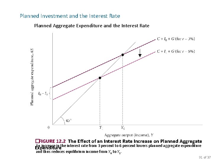
Planned Investment and the Interest Rate Planned Aggregate Expenditure and the Interest Rate �FIGURE 12. 2 The Effect of an Interest Rate Increase on Planned Aggregate An increase in the interest rate from 3 percent to 6 percent lowers planned aggregate expenditure Expenditure and thus reduces equilibrium income from Y 0 to Y 1. 91 of 37

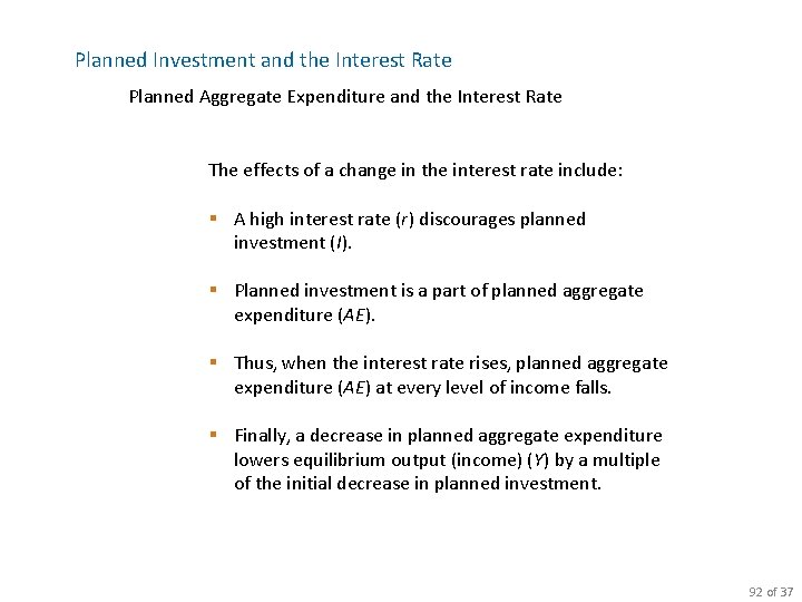
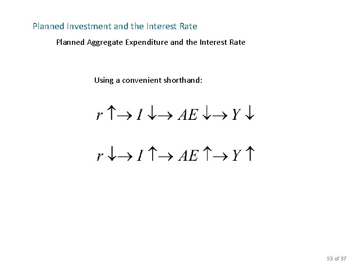
Planned Investment and the Interest Rate Planned Aggregate Expenditure and the Interest Rate The effects of a change in the interest rate include: § A high interest rate (r) discourages planned investment (I). § Planned investment is a part of planned aggregate expenditure (AE). § Thus, when the interest rate rises, planned aggregate expenditure (AE) at every level of income falls. § Finally, a decrease in planned aggregate expenditure lowers equilibrium output (income) (Y) by a multiple of the initial decrease in planned investment. 92 of 37

Planned Investment and the Interest Rate Planned Aggregate Expenditure and the Interest Rate Using a convenient shorthand: 93 of 37

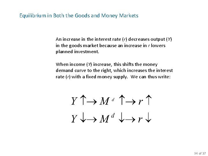
Equilibrium in Both the Goods and Money Markets An increase in the interest rate (r) decreases output (Y) in the goods market because an increase in r lowers planned investment. When income (Y) increase, this shifts the money demand curve to the right, which increases the interest rate (r) with a fixed money supply. We can thus write: 94 of 37

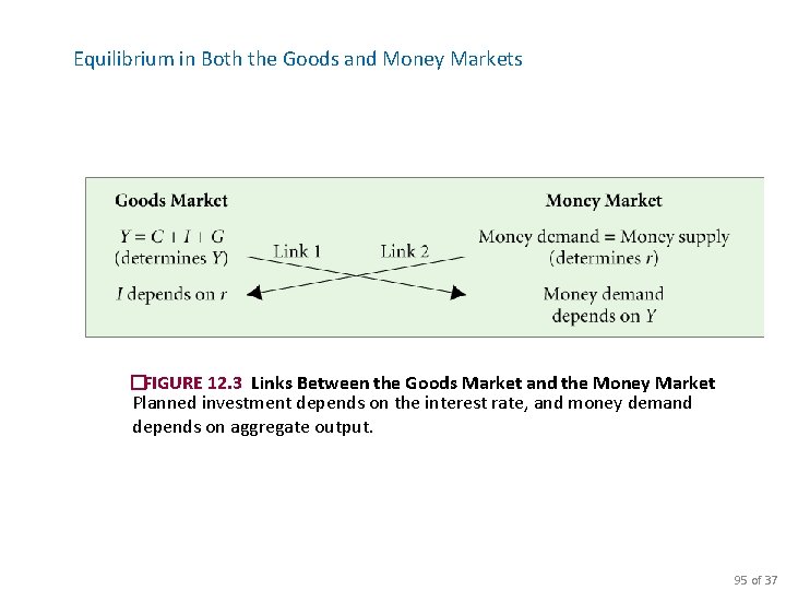
Equilibrium in Both the Goods and Money Markets �FIGURE 12. 3 Links Between the Goods Market and the Money Market Planned investment depends on the interest rate, and money demand depends on aggregate output. 95 of 37

Policy Effects in the Goods and Money Markets Expansionary Policy Effects expansionary fiscal policy An increase in government spending or a reduction in net taxes aimed at increasing aggregate output (income) (Y). expansionary monetary policy An increase in the money supply aimed at increasing aggregate output (income) (Y). 96 of 37

Policy Effects in the Goods and Money Markets Expansionary Policy Effects Expansionary Fiscal Policy: An Increase in Government Purchases (G) or a Decrease in Net Taxes (T) crowding-out effect The tendency for increases in government spending to cause reductions in private investment spending. 97 of 37

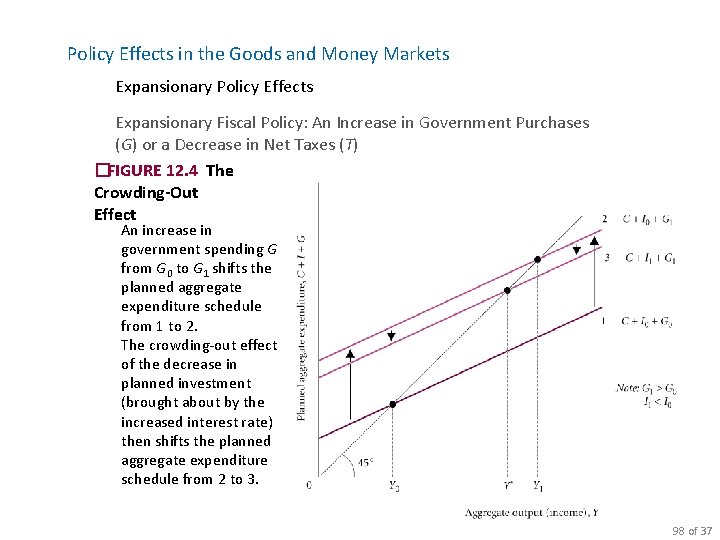
Policy Effects in the Goods and Money Markets Expansionary Policy Effects Expansionary Fiscal Policy: An Increase in Government Purchases (G) or a Decrease in Net Taxes (T) �FIGURE 12. 4 The Crowding-Out Effect An increase in government spending G from G 0 to G 1 shifts the planned aggregate expenditure schedule from 1 to 2. The crowding-out effect of the decrease in planned investment (brought about by the increased interest rate) then shifts the planned aggregate expenditure schedule from 2 to 3. 98 of 37

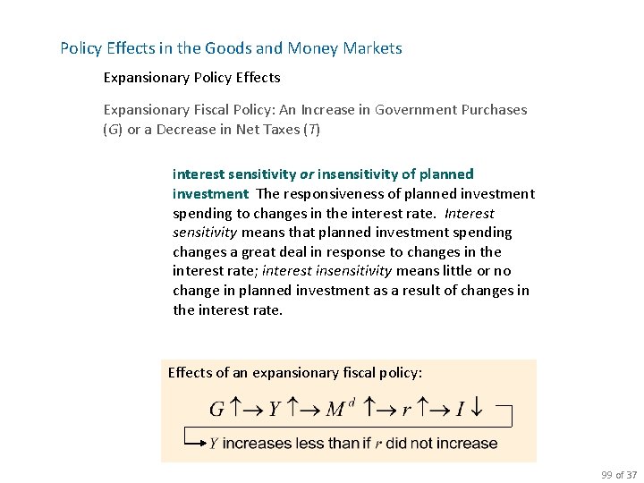
Policy Effects in the Goods and Money Markets Expansionary Policy Effects Expansionary Fiscal Policy: An Increase in Government Purchases (G) or a Decrease in Net Taxes (T) interest sensitivity or insensitivity of planned investment The responsiveness of planned investment spending to changes in the interest rate. Interest sensitivity means that planned investment spending changes a great deal in response to changes in the interest rate; interest insensitivity means little or no change in planned investment as a result of changes in the interest rate. Effects of an expansionary fiscal policy: 99 of 37

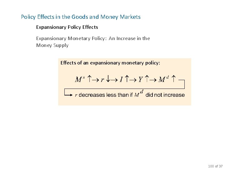
Policy Effects in the Goods and Money Markets Expansionary Policy Effects Expansionary Monetary Policy: An Increase in the Money Supply Effects of an expansionary monetary policy: 100 of 37

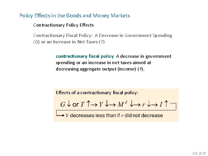
Policy Effects in the Goods and Money Markets Contractionary Policy Effects Contractionary Fiscal Policy: A Decrease in Government Spending (G) or an Increase in Net Taxes (T) contractionary fiscal policy A decrease in government spending or an increase in net taxes aimed at decreasing aggregate output (income) (Y). Effects of a contractionary fiscal policy: 101 of 37

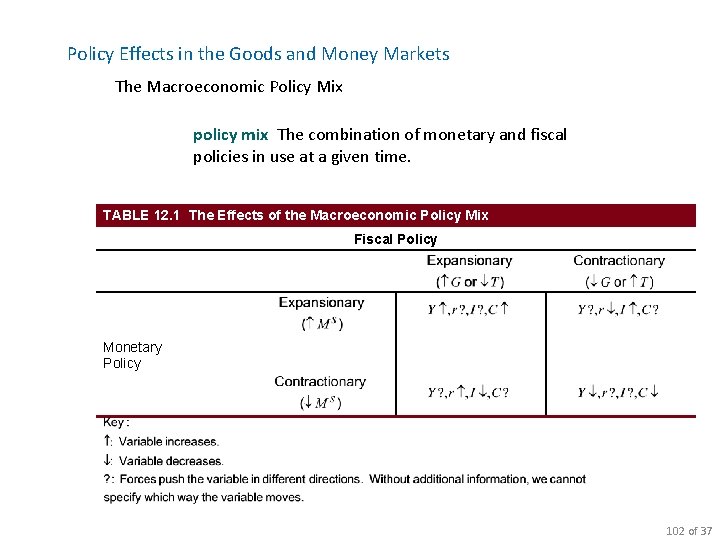
Policy Effects in the Goods and Money Markets The Macroeconomic Policy Mix policy mix The combination of monetary and fiscal policies in use at a given time. TABLE 12. 1 The Effects of the Macroeconomic Policy Mix Fiscal Policy Monetary Policy 102 of 37

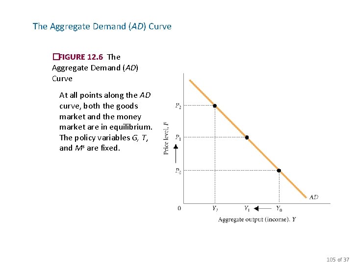
The Aggregate Demand (AD) Curve aggregate demand The total demand for goods and services in the economy. aggregate demand (AD) curve A curve that shows the negative relationship between aggregate output (income) and the price level. Each point on the AD curve is a point at which both the goods market and the money market are in equilibrium. 103 of 37

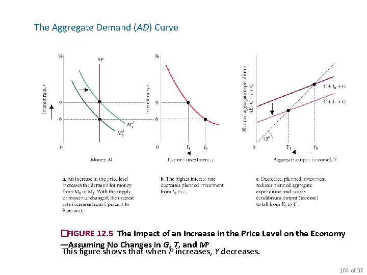
The Aggregate Demand (AD) Curve �FIGURE 12. 5 The Impact of an Increase in the Price Level on the Economy —Assuming No Changes in G, T, and Ms This figure shows that when P increases, Y decreases. 104 of 37

The Aggregate Demand (AD) Curve �FIGURE 12. 6 The Aggregate Demand (AD) Curve At all points along the AD curve, both the goods market and the money market are in equilibrium. The policy variables G, T, and Ms are fixed. 105 of 37

The Aggregate Demand (AD) Curve The Aggregate Demand Curve: A Warning It is important that you realize what the aggregate demand curve represents. The aggregate demand curve is more complex than a simple individual or market demand curve. The AD curve is not a market demand curve, and it is not the sum of all market demand curves in the economy. To understand what the aggregate demand curve represents, you must understand the interaction between the goods market and the money markets. 106 of 37

The Aggregate Demand (AD) Curve Other Reasons for a Downward-Sloping Aggregate Demand Curve The Consumption Link The consumption link provides another reason for the AD curve’s downward slope. An increase in the price level increases the demand for money, which leads to an increase in the interest rate, which leads to a decrease in consumption (as well as planned investment), which leads to a decrease in aggregate output (income). 107 of 37

The Aggregate Demand (AD) Curve Other Reasons for a Downward-Sloping Aggregate Demand Curve The Consumption Link The initial decrease in consumption (brought about by the increase in the interest rate) contributes to the overall decrease in output. Planned investment does not bear all the burden of providing the link from a higher interest rate to a lower level of aggregate output. Decreased consumption brought about by a higher interest rate also contributes to this effect. 108 of 37

The Aggregate Demand (AD) Curve Other Reasons for a Downward-Sloping Aggregate Demand Curve The Real Wealth Effect real wealth, or real balance, effect The change in consumption brought about by a change in real wealth that results from a change in the price level. 109 of 37

The Aggregate Demand (AD) Curve Aggregate Expenditure and Aggregate Demand At equilibrium, planned aggregate expenditure (AE ≡ C + I + G) and aggregate output (Y) are equal: equilibrium condition: C + I + G = Y 110 of 37

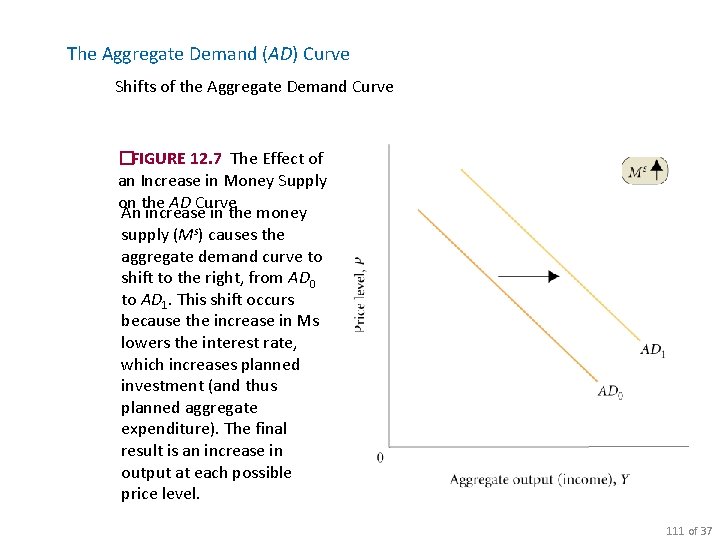
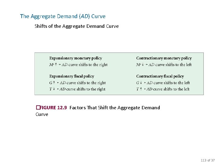
The Aggregate Demand (AD) Curve Shifts of the Aggregate Demand Curve �FIGURE 12. 7 The Effect of an Increase in Money Supply on the AD Curve An increase in the money supply (Ms) causes the aggregate demand curve to shift to the right, from AD 0 to AD 1. This shift occurs because the increase in Ms lowers the interest rate, which increases planned investment (and thus planned aggregate expenditure). The final result is an increase in output at each possible price level. 111 of 37

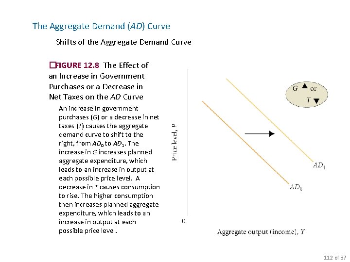
The Aggregate Demand (AD) Curve Shifts of the Aggregate Demand Curve �FIGURE 12. 8 The Effect of an Increase in Government Purchases or a Decrease in Net Taxes on the AD Curve An increase in government purchases (G) or a decrease in net taxes (T) causes the aggregate demand curve to shift to the right, from AD 0 to AD 1. The increase in G increases planned aggregate expenditure, which leads to an increase in output at each possible price level. A decrease in T causes consumption to rise. The higher consumption then increases planned aggregate expenditure, which leads to an increase in output at each possible price level. 112 of 37

The Aggregate Demand (AD) Curve Shifts of the Aggregate Demand Curve �FIGURE 12. 9 Factors That Shift the Aggregate Demand Curve 113 of 37

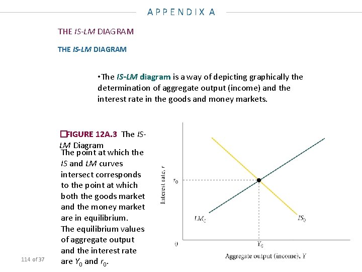
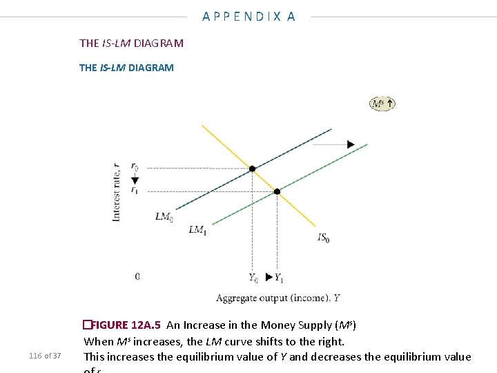
APPENDIX A THE IS-LM DIAGRAM • The IS-LM diagram is a way of depicting graphically the determination of aggregate output (income) and the interest rate in the goods and money markets. 114 of 37 �FIGURE 12 A. 3 The ISLM Diagram The point at which the IS and LM curves intersect corresponds to the point at which both the goods market and the money market are in equilibrium. The equilibrium values of aggregate output and the interest rate are Y 0 and r 0.

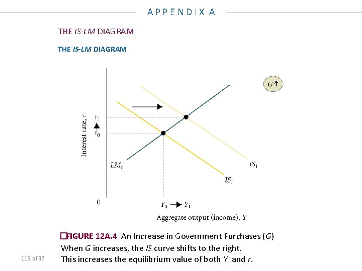
APPENDIX A THE IS-LM DIAGRAM 115 of 37 �FIGURE 12 A. 4 An Increase in Government Purchases (G) When G increases, the IS curve shifts to the right. This increases the equilibrium value of both Y and r.

APPENDIX A THE IS-LM DIAGRAM 116 of 37 �FIGURE 12 A. 5 An Increase in the Money Supply (Ms) When Ms increases, the LM curve shifts to the right. This increases the equilibrium value of Y and decreases the equilibrium value

The Aggregate Supply Curve aggregate supply The total supply of all goods and services in an economy. The Aggregate Supply Curve: A Warning aggregate supply (AS) curve A graph that shows the relationship between the aggregate quantity of output supplied by all firms in an economy and the overall price level. An “aggregate supply curve” in the traditional sense of the word supply does not exist. What does exist is what we might call a “price/output response” curve—a curve that traces out the price decisions and output decisions of all firms in the economy under a given set of circumstances. 117 of 25

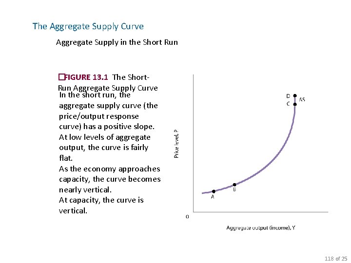
The Aggregate Supply Curve Aggregate Supply in the Short Run �FIGURE 13. 1 The Short. Run Aggregate Supply Curve In the short run, the aggregate supply curve (the price/output response curve) has a positive slope. At low levels of aggregate output, the curve is fairly flat. As the economy approaches capacity, the curve becomes nearly vertical. At capacity, the curve is vertical. 118 of 25

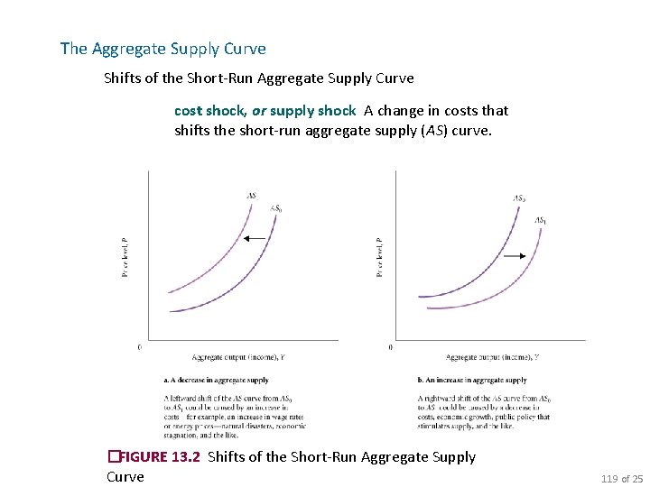
The Aggregate Supply Curve Shifts of the Short-Run Aggregate Supply Curve cost shock, or supply shock A change in costs that shifts the short-run aggregate supply (AS) curve. �FIGURE 13. 2 Shifts of the Short-Run Aggregate Supply Curve 119 of 25

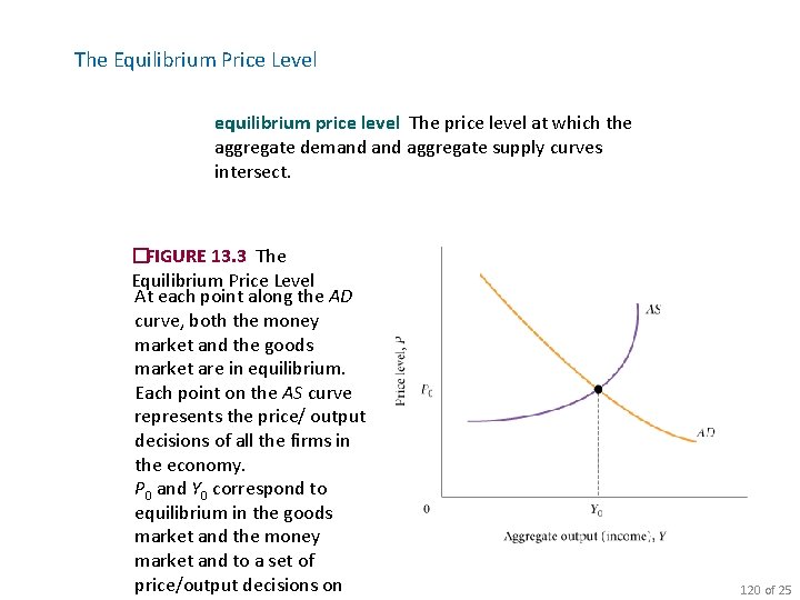
The Equilibrium Price Level equilibrium price level The price level at which the aggregate demand aggregate supply curves intersect. �FIGURE 13. 3 The Equilibrium Price Level At each point along the AD curve, both the money market and the goods market are in equilibrium. Each point on the AS curve represents the price/ output decisions of all the firms in the economy. P 0 and Y 0 correspond to equilibrium in the goods market and the money market and to a set of price/output decisions on 120 of 25

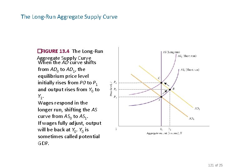
The Long-Run Aggregate Supply Curve �FIGURE 13. 4 The Long-Run Aggregate Supply Curve When the AD curve shifts from AD 0 to AD 1, the equilibrium price level initially rises from P 0 to P 1 and output rises from Y 0 to Y 1. Wages respond in the longer run, shifting the AS curve from AS 0 to AS 1. If wages fully adjust, output will be back at Y 0 is sometimes called potential GDP. 121 of 25

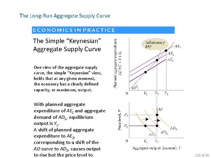
The Long-Run Aggregate Supply Curve The Simple “Keynesian” Aggregate Supply Curve One view of the aggregate supply curve, the simple “Keynesian” view, holds that at any given moment, the economy has a clearly defined capacity, or maximum, output. With planned aggregate expenditure of AE 1 and aggregate demand of AD 1, equilibrium output is Y 1. A shift of planned aggregate expenditure to AE 2, corresponding to a shift of the AD curve to AD 2, causes output to rise but the price level to 122 of 25

The Long-Run Aggregate Supply Curve Potential GDP potential output, or potential GDP The level of aggregate output that can be sustained in the long run without inflation. Short-Run Equilibrium Below Potential Output Although different economists have different opinions on how to determine whether an economy is operating at or above potential output, there is general agreement that there is a maximum level of output (below the vertical portion of the short-run aggregate supply curve) that can be sustained without inflation. 123 of 25

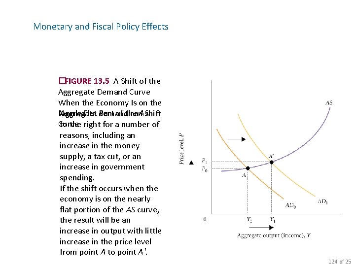
Monetary and Fiscal Policy Effects �FIGURE 13. 5 A Shift of the Aggregate Demand Curve When the Economy Is on the Nearly Flat demand Part of the Aggregate can. ASshift Curve to the right for a number of reasons, including an increase in the money supply, a tax cut, or an increase in government spending. If the shift occurs when the economy is on the nearly flat portion of the AS curve, the result will be an increase in output with little increase in the price level from point A to point A’. 124 of 25

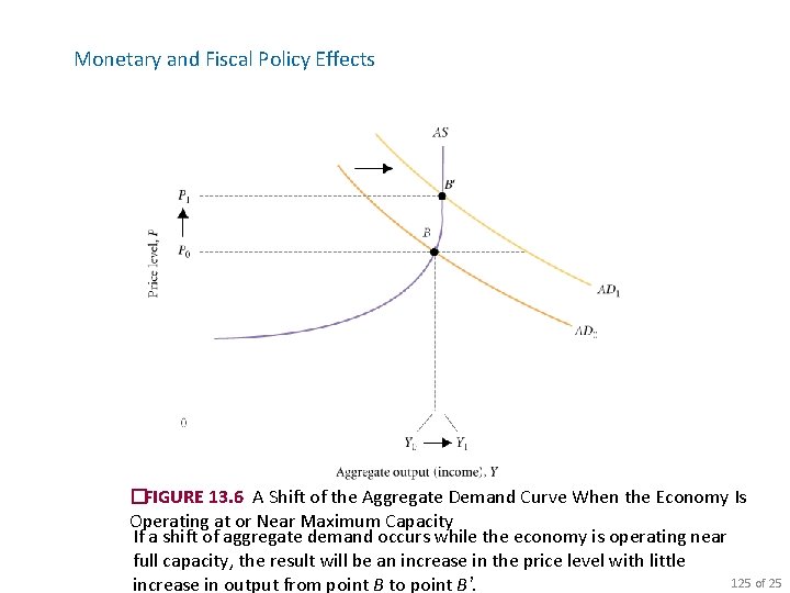
Monetary and Fiscal Policy Effects �FIGURE 13. 6 A Shift of the Aggregate Demand Curve When the Economy Is Operating at or Near Maximum Capacity If a shift of aggregate demand occurs while the economy is operating near full capacity, the result will be an increase in the price level with little 125 of 25 increase in output from point B to point B’.

Monetary and Fiscal Policy Effects Long-Run Aggregate Supply and Policy Effects It is important to realize that if the AS curve is vertical in the long run, neither monetary policy nor fiscal policy has any effect on aggregate output in the long run. The conclusion that policy has no effect on aggregate output in the long run is perhaps startling. 126 of 25

Causes of Inflation Demand-Pull Inflation demand-pull inflation Inflation that is initiated by an increase in aggregate demand. 127 of 25

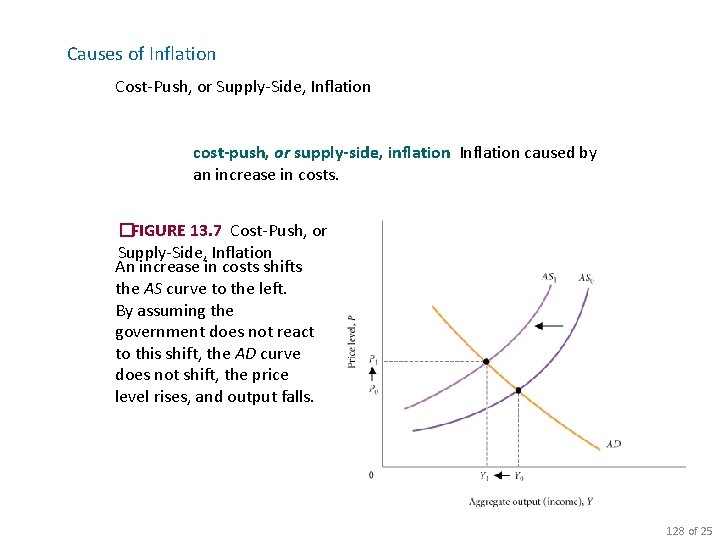
Causes of Inflation Cost-Push, or Supply-Side, Inflation cost-push, or supply-side, inflation Inflation caused by an increase in costs. �FIGURE 13. 7 Cost-Push, or Supply-Side, Inflation An increase in costs shifts the AS curve to the left. By assuming the government does not react to this shift, the AD curve does not shift, the price level rises, and output falls. 128 of 25

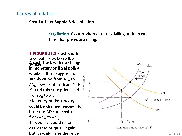
Causes of Inflation Cost-Push, or Supply-Side, Inflation stagflation Occurs when output is falling at the same time that prices are rising. �FIGURE 13. 8 Cost Shocks Are Bad News for Policy AMakers cost shock with no change in monetary or fiscal policy would shift the aggregate supply curve from AS 0 to AS 1, lower output from Y 0 to Y 1, and raise the price level from P 0 to P 1. Monetary or fiscal policy could be changed enough to have the AD curve shift from AD 0 to AD 1. This policy would raise aggregate output Y again, but it would raise the price 129 of 25

Causes of Inflation Expectations and Inflation When firms are making their price/output decisions, their expectations of future prices may affect their current decisions. If a firm expects that its competitors will raise their prices, in anticipation, it may raise its own price. Given the importance of expectations in inflation, the central banks of many countries survey consumers about their expectations. 130 of 25

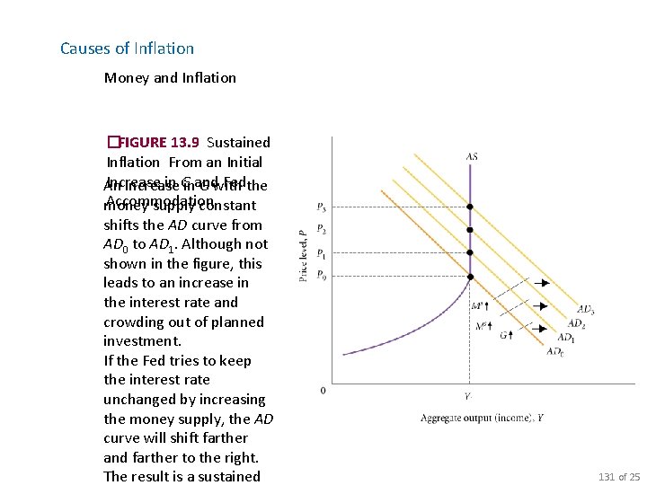
Causes of Inflation Money and Inflation �FIGURE 13. 9 Sustained Inflation From an Initial Increase in Ginand Fedthe An increase G with Accommodation money supply constant shifts the AD curve from AD 0 to AD 1. Although not shown in the figure, this leads to an increase in the interest rate and crowding out of planned investment. If the Fed tries to keep the interest rate unchanged by increasing the money supply, the AD curve will shift farther and farther to the right. The result is a sustained 131 of 25

Causes of Inflation Sustained Inflation as a Purely Monetary Phenomenon Virtually all economists agree that an increase in the price level can be caused by anything that causes the AD curve to shift to the right or the AS curve to shift to the left. It is also generally agreed that for a sustained inflation to occur, the Fed must accommodate it. In this sense, a sustained inflation can be thought of as a purely monetary phenomenon. 132 of 25

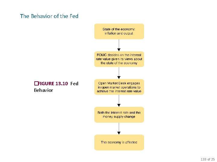
The Behavior of the Fed �FIGURE 13. 10 Fed Behavior 133 of 25

The Behavior of the Fed Controlling the Interest Rate The buying and selling of government securities by the Fed has two effects at the same time: It changes the money supply, and it changes the interest rate. How much the interest rate changes depends on the shape of the money demand curve. The steeper the money demand curve, the larger the change in the interest rate for a given size change in government securities. If the Fed wants to achieve a particular value of the money supply, it must accept whatever interest rate value is implied by this choice. Conversely, if the Fed wants to achieve a particular value of the interest rate, it must accept whatever money supply value is implied by this. 134 of 25

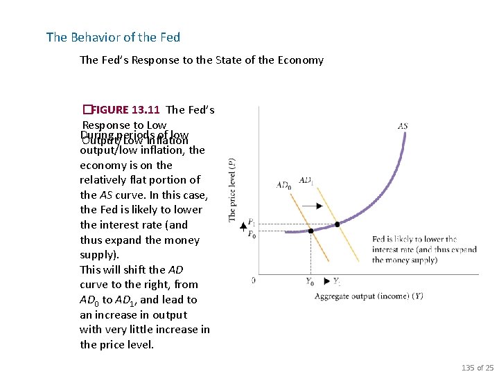
The Behavior of the Fed The Fed’s Response to the State of the Economy �FIGURE 13. 11 The Fed’s Response to Low During periods of low Output/Low Inflation output/low inflation, the economy is on the relatively flat portion of the AS curve. In this case, the Fed is likely to lower the interest rate (and thus expand the money supply). This will shift the AD curve to the right, from AD 0 to AD 1, and lead to an increase in output with very little increase in the price level. 135 of 25

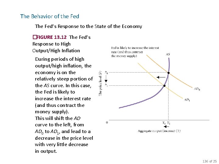
The Behavior of the Fed The Fed’s Response to the State of the Economy �FIGURE 13. 12 The Fed’s Response to High Output/High Inflation During periods of high output/high inflation, the economy is on the relatively steep portion of the AS curve. In this case, the Fed is likely to increase the interest rate (and thus contract the money supply). This will shift the AD curve to the left, from AD 0 to AD 1, and lead to a decrease in the price level with very little decrease in output. 136 of 25

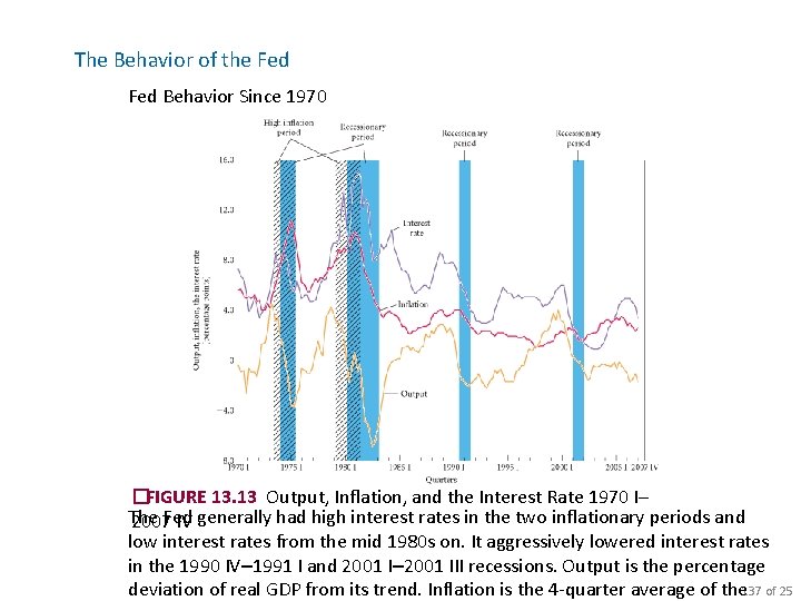
The Behavior of the Fed Behavior Since 1970 �FIGURE 13. 13 Output, Inflation, and the Interest Rate 1970 I– The 2007 Fed IV generally had high interest rates in the two inflationary periods and low interest rates from the mid 1980 s on. It aggressively lowered interest rates in the 1990 IV– 1991 I and 2001 I– 2001 III recessions. Output is the percentage deviation of real GDP from its trend. Inflation is the 4 -quarter average of the 137 of 25

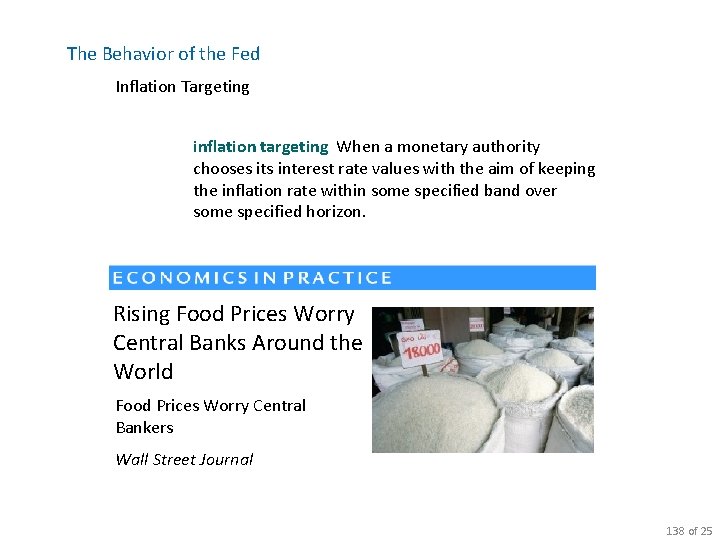
The Behavior of the Fed Inflation Targeting inflation targeting When a monetary authority chooses its interest rate values with the aim of keeping the inflation rate within some specified band over some specified horizon. Rising Food Prices Worry Central Banks Around the World Food Prices Worry Central Bankers Wall Street Journal 138 of 25

The Labor Market: Basic Concepts frictional unemployment The portion of unemployment that is due to the normal working of the labor market; used to denote short-run job/skill matching problems. structural unemployment The portion of unemployment that is due to changes in the structure of the economy that result in a significant loss of jobs in certain industries. cyclical unemployment The increase in unemployment that occurs during recessions and depressions. 139 of 29

The Classical View of the Labor Market labor demand curve A graph that illustrates the amount of labor that firms want to employ at each given wage rate. labor supply curve A graph that illustrates the amount of labor that households want to supply at each given wage rate. 140 of 29

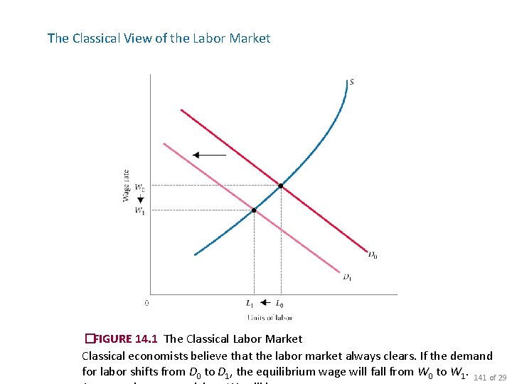
The Classical View of the Labor Market �FIGURE 14. 1 The Classical Labor Market Classical economists believe that the labor market always clears. If the demand for labor shifts from D 0 to D 1, the equilibrium wage will fall from W 0 to W 1. 141 of 29

The Classical View of the Labor Market The Classical Labor Market and the Aggregate Supply Curve The classical idea that wages adjust to clear the labor market is consistent with the view that wages respond quickly to price changes. This means that the AS curve is vertical. When the AS curve is vertical, monetary and fiscal policy cannot affect the level of output and employment in the economy. 142 of 29

The Classical View of the Labor Market The Unemployment Rate and the Classical View The unemployment rate is not necessarily an accurate indicator of whether the labor market is working properly. The measured unemployment rate may sometimes seem high even though the labor market is working well. 143 of 29

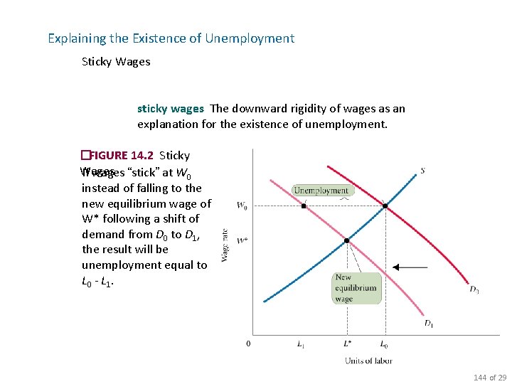
Explaining the Existence of Unemployment Sticky Wages sticky wages The downward rigidity of wages as an explanation for the existence of unemployment. �FIGURE 14. 2 Sticky Wages If wages “stick” at W 0 instead of falling to the new equilibrium wage of W* following a shift of demand from D 0 to D 1, the result will be unemployment equal to L 0 - L 1. 144 of 29

Explaining the Existence of Unemployment Sticky Wages Social, or Implicit, Contracts social, or implicit, contracts Unspoken agreements between workers and firms that firms will not cut wages. relative-wage explanation of unemployment An explanation for sticky wages (and therefore unemployment): If workers are concerned about their wages relative to other workers in other firms and industries, they may be unwilling to accept a wage cut unless they know that all other workers are receiving similar cuts. 145 of 29

Explaining the Existence of Unemployment Sticky Wages Explicit Contracts explicit contracts Employment contracts that stipulate workers’ wages, usually for a period of 1 to 3 years. cost-of-living adjustments (COLAs) Contract provisions that tie wages to changes in the cost of living. The greater the inflation rate, the more wages are raised. 146 of 29

Explaining the Existence of Unemployment Sticky Wages Explicit Contracts Graduate School Applications in Recessions Graduate School Offers Relief During Economic Recession Oklahoma Daily (U. Oklahoma) 147 of 29

Explaining the Existence of Unemployment Efficiency Wage Theory efficiency wage theory An explanation for unemployment that holds that the productivity of workers increases with the wage rate. If this is so, firms may have an incentive to pay wages above the marketclearing rate. 148 of 29

Explaining the Existence of Unemployment Imperfect Information Firms may not have enough information at their disposal to know what the market-clearing wage is. In this case, firms are said to have imperfect information. If firms have imperfect or incomplete information, they may set wages wrong—wages that do not clear the labor market. 149 of 29

Explaining the Existence of Unemployment Minimum Wage Laws minimum wage laws Laws that set a floor for wage rates—that is, a minimum hourly rate for any kind of labor. An Open Question The aggregate labor market is very complicated, and there are no simple answers to why there is unemployment. 150 of 29

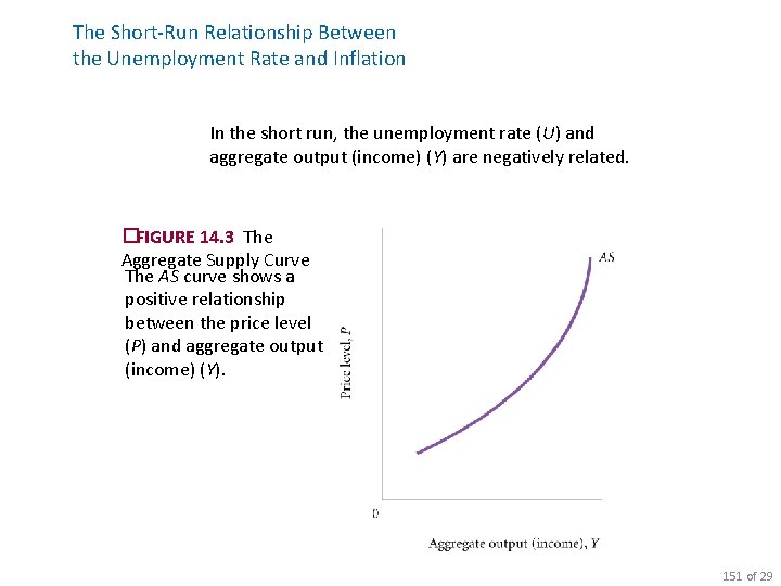
The Short-Run Relationship Between the Unemployment Rate and Inflation In the short run, the unemployment rate (U) and aggregate output (income) (Y) are negatively related. �FIGURE 14. 3 The Aggregate Supply Curve The AS curve shows a positive relationship between the price level (P) and aggregate output (income) (Y). 151 of 29

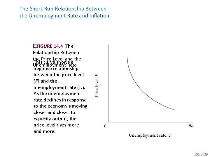
The Short-Run Relationship Between the Unemployment Rate and Inflation �FIGURE 14. 4 The Relationship Between the Price Level and the This curve shows a Unemployment Rate negative relationship between the price level (P) and the unemployment rate (U). As the unemployment rate declines in response to the economy’s moving closer and closer to capacity output, the price level rises more and more. 152 of 29

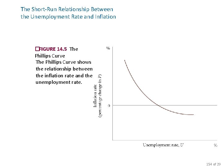
The Short-Run Relationship Between the Unemployment Rate and Inflation inflation rate The percentage change in the price level. Phillips Curve A curve showing the relationship between the inflation rate and the unemployment rate. 153 of 29

The Short-Run Relationship Between the Unemployment Rate and Inflation �FIGURE 14. 5 The Phillips Curve shows the relationship between the inflation rate and the unemployment rate. 154 of 29

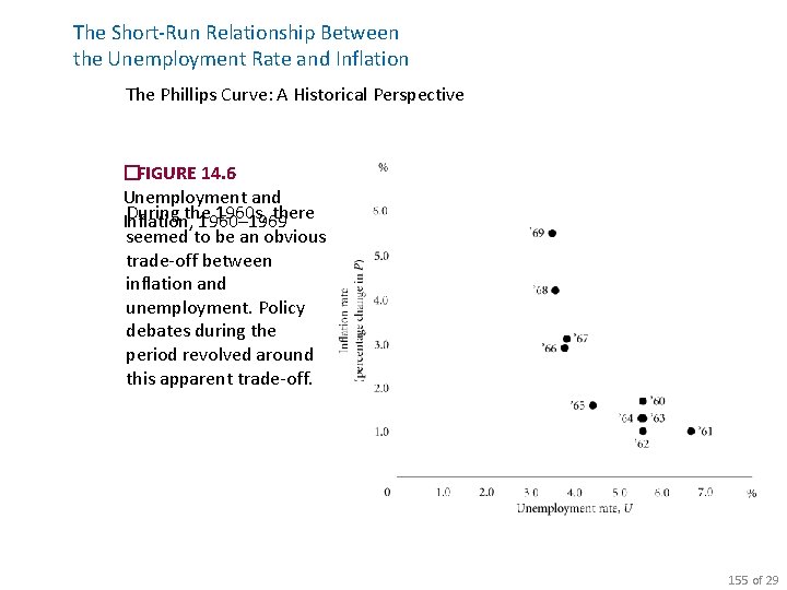
The Short-Run Relationship Between the Unemployment Rate and Inflation The Phillips Curve: A Historical Perspective �FIGURE 14. 6 Unemployment and During the 1960 s, there Inflation, 1960– 1969 seemed to be an obvious trade-off between inflation and unemployment. Policy debates during the period revolved around this apparent trade-off. 155 of 29

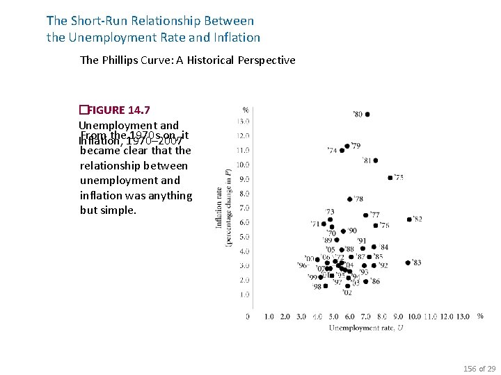
The Short-Run Relationship Between the Unemployment Rate and Inflation The Phillips Curve: A Historical Perspective �FIGURE 14. 7 Unemployment and From the 1970– 2007 1970 s on, it Inflation, became clear that the relationship between unemployment and inflation was anything but simple. 156 of 29

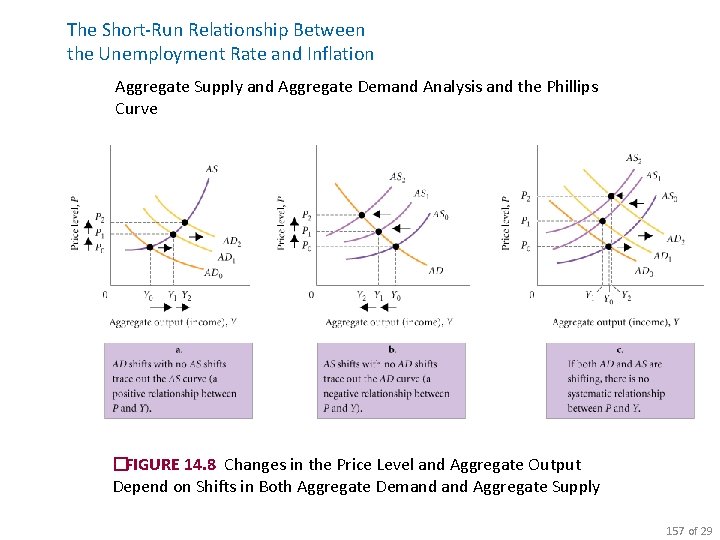
The Short-Run Relationship Between the Unemployment Rate and Inflation Aggregate Supply and Aggregate Demand Analysis and the Phillips Curve �FIGURE 14. 8 Changes in the Price Level and Aggregate Output Depend on Shifts in Both Aggregate Demand Aggregate Supply 157 of 29

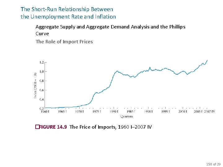
The Short-Run Relationship Between the Unemployment Rate and Inflation Aggregate Supply and Aggregate Demand Analysis and the Phillips Curve The Role of Import Prices �FIGURE 14. 9 The Price of Imports, 1960 I– 2007 IV 158 of 29

The Short-Run Relationship Between the Unemployment Rate and Inflation Expectations and the Phillips Curve Expectations are self-fulfilling. This means that wage inflation is affected by expectations of future price inflation. Price expectations that affect wage contracts eventually affect prices themselves. Inflationary expectations shift the Phillips Curve to the right. 159 of 29

The Short-Run Relationship Between the Unemployment Rate and Inflation Is There a Short-Run Trade-Off between Inflation and Unemployment? There is a short-run trade-off between inflation and unemployment, but other factors besides unemployment affect inflation. Policy involves more than simply choosing a point along a nice smooth curve. 160 of 29

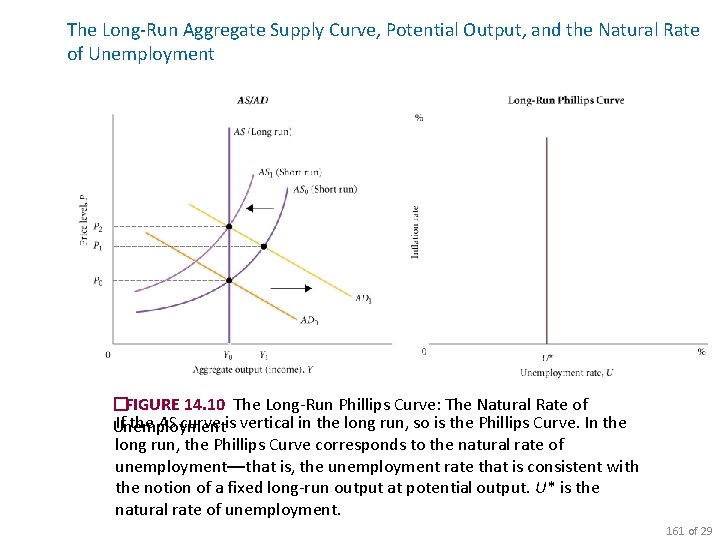
The Long-Run Aggregate Supply Curve, Potential Output, and the Natural Rate of Unemployment �FIGURE 14. 10 The Long-Run Phillips Curve: The Natural Rate of If the AS curve is vertical in the long run, so is the Phillips Curve. In the Unemployment long run, the Phillips Curve corresponds to the natural rate of unemployment—that is, the unemployment rate that is consistent with the notion of a fixed long-run output at potential output. U* is the natural rate of unemployment. 161 of 29

Time Lags Regarding Monetary and Fiscal Policy stabilization policy Describes both monetary and fiscal policy, the goals of which are to smooth out fluctuations in output and employment and to keep prices as stable as possible. time lags Delays in the economy’s response to stabilization policies. 162 of 31

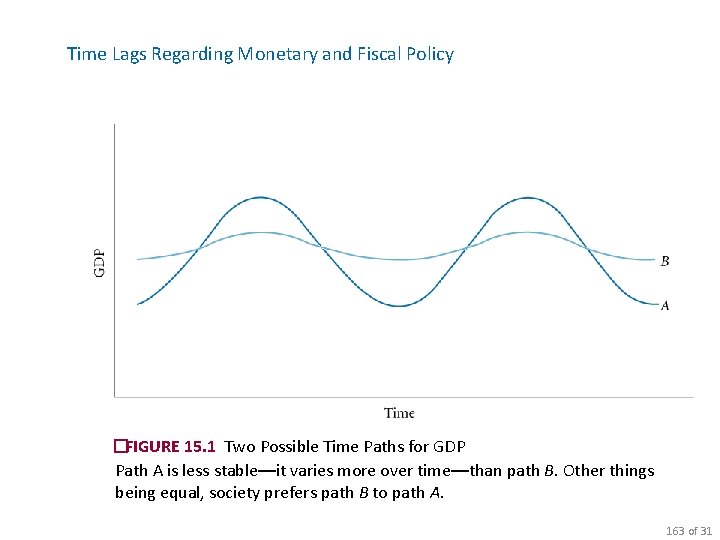
Time Lags Regarding Monetary and Fiscal Policy �FIGURE 15. 1 Two Possible Time Paths for GDP Path A is less stable—it varies more over time—than path B. Other things being equal, society prefers path B to path A. 163 of 31

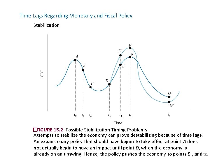
Time Lags Regarding Monetary and Fiscal Policy Stabilization �FIGURE 15. 2 Possible Stabilization Timing Problems Attempts to stabilize the economy can prove destabilizing because of time lags. An expansionary policy that should have begun to take effect at point A does not actually begin to have an impact until point D, when the economy is 164 of 31 already on an upswing. Hence, the policy pushes the economy to points E 1, and

Time Lags Regarding Monetary and Fiscal Policy Recognition Lags recognition lag The time it takes for policy makers to recognize the existence of a boom or a slump. Implementation Lags implementation lag The time it takes to put the desired policy into effect once economists and policy makers recognize that the economy is in a boom or a slump. 165 of 31

Time Lags Regarding Monetary and Fiscal Policy Response Lags response lag The time that it takes for the economy to adjust to the new conditions after a new policy is implemented; the lag that occurs because of the operation of the economy itself. 166 of 31

Time Lags Regarding Monetary and Fiscal Policy Response Lags for Fiscal Policy Neither individuals nor firms revise their spending plans instantaneously. Until they can make those revisions, extra government spending does not stimulate extra private spending. Response Lags for Monetary Policy Monetary policy works by changing interest rates, which then change planned investment. The response of consumption and investment to interest rate changes takes time. 167 of 31

Time Lags Regarding Monetary and Fiscal Policy Response Lags Summary Stabilization is not easily achieved. It takes time for policy makers to recognize the existence of a problem, more time for them to implement a solution, and yet more time for firms and households to respond to the stabilization policies taken. 168 of 31

Fiscal Policy: Deficit Targeting Gramm-Rudman-Hollings Act Passed by the U. S. Congress and signed by President Reagan in 1986, this law set out to reduce the federal deficit by $36 billion per year, with a deficit of zero slated for 1991. �FIGURE 15. 3 Deficit Reduction Targets under Gramm-Rudman-Hollings The GRH legislation, passed in 1986, set out to lower the federal deficit by $36 billion per year. If the plan had worked, a zero deficit would have been achieved by 1991. 169 of 31

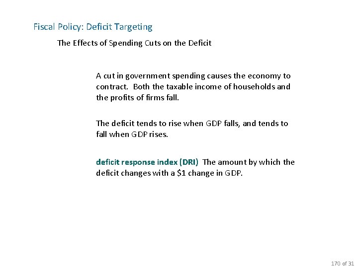
Fiscal Policy: Deficit Targeting The Effects of Spending Cuts on the Deficit A cut in government spending causes the economy to contract. Both the taxable income of households and the profits of firms fall. The deficit tends to rise when GDP falls, and tends to fall when GDP rises. deficit response index (DRI) The amount by which the deficit changes with a $1 change in GDP. 170 of 31

Fiscal Policy: Deficit Targeting The Effects of Spending Cuts on the Deficit Monetary Policy to the Rescue? A zero multiplier can come about through renewed optimism on the part of households and firms or through very aggressive behavior on the part of the Fed, but because neither of these situations is very plausible, the multiplier is likely to be greater than zero. Thus, it is likely that to lower the deficit by a certain amount, the cut in government spending must be larger than that amount. 171 of 31

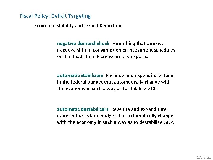
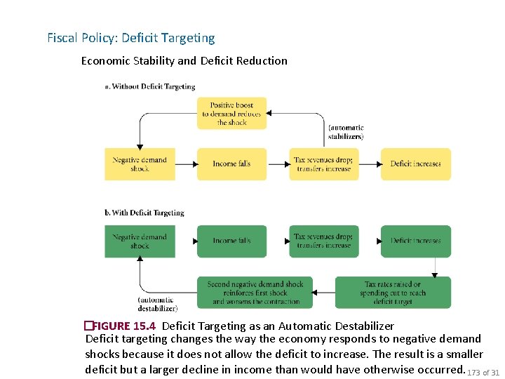
Fiscal Policy: Deficit Targeting Economic Stability and Deficit Reduction negative demand shock Something that causes a negative shift in consumption or investment schedules or that leads to a decrease in U. S. exports. automatic stabilizers Revenue and expenditure items in the federal budget that automatically change with the economy in such a way as to stabilize GDP. automatic destabilizers Revenue and expenditure items in the federal budget that automatically change with the economy in such a way as to destabilize GDP. 172 of 31

Fiscal Policy: Deficit Targeting Economic Stability and Deficit Reduction �FIGURE 15. 4 Deficit Targeting as an Automatic Destabilizer Deficit targeting changes the way the economy responds to negative demand shocks because it does not allow the deficit to increase. The result is a smaller deficit but a larger decline in income than would have otherwise occurred. 173 of 31

Fiscal Policy: Deficit Targeting Summary It is clear that the GRH legislation, the balanced-budget amendment, and similar deficit targeting measures have some undesirable macroeconomic consequences. Locking the economy into spending cuts during periods of negative demand shocks, as deficit-targeting measures do, is not a good way to manage the economy. 174 of 31

Long-Run Growth economic growth An increase in the total output of an economy. modern economic growth The period of rapid and sustained increase in output that began in the Western world with the Industrial Revolution. 175 of 27

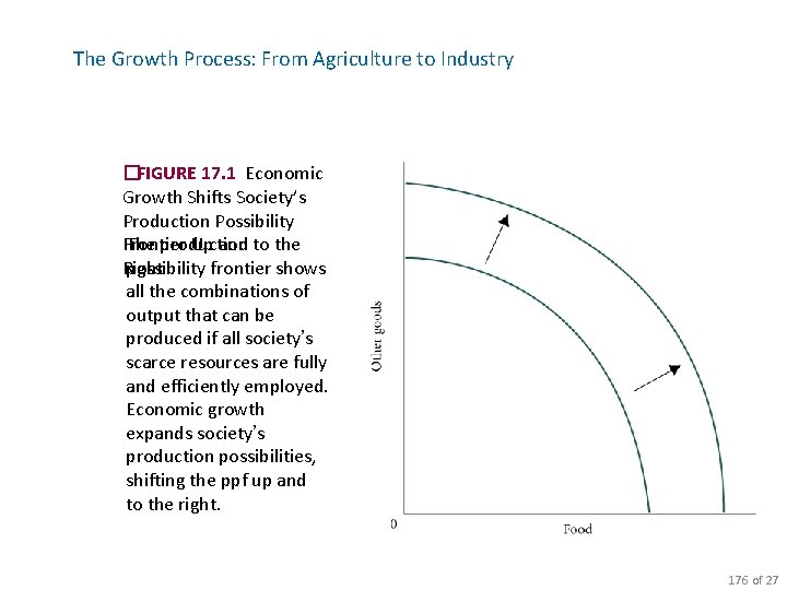
The Growth Process: From Agriculture to Industry �FIGURE 17. 1 Economic Growth Shifts Society’s Production Possibility The production Frontier Up and to the possibility frontier shows Right all the combinations of output that can be produced if all society’s scarce resources are fully and efficiently employed. Economic growth expands society’s production possibilities, shifting the ppf up and to the right. 176 of 27

The Growth Process: From Agriculture to Industry: The Industrial Revolution Beginning in England around 1750, technical change and capital accumulation increased productivity significantly in two important industries: agriculture and textiles. More could be produced with fewer resources, leading to new products, more output, and wider choice. A rural agrarian society was very quickly transformed into an urban industrial society. 177 of 27

The Growth Process: From Agriculture to Industry Growth in Modern Society Economic growth continues today, and while the underlying process is still the same, the face is different. Growth comes from a bigger workforce and more productive workers. Higher productivity comes from tools (capital), a better-educated and more highly skilled workforce (human capital), and increasingly from innovation and technical change (new techniques of production) and newly developed products and services. 178 of 27

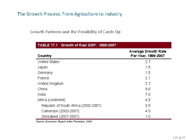
The Growth Process: From Agriculture to Industry Growth Patterns and the Possibility of Catch-Up TABLE 17. 1 Growth of Real GDP: 1999 -2007 Country Average Growth Rate Per Year, 1999 -2007 United States 2. 7 Japan 1. 5 Germany 1. 5 France 2. 1 United Kingdom 2. 7 China 9. 6 India 7. 0 Africa (continent) 4. 5 Republic of South Africa (2002 -2007) 3. 9 Cameroon (2002 -2007) 4. 0 Zimbabwe (2007 -2007) 1. 0 Source: Economic Report of the President, 2008. 179 of 27

The Growth Process: From Agriculture to Industry Growth Patterns and the Possibility of Catch-Up catch-up The theory stating that the growth rates of less developed countries will exceed the growth rates of developed countries, allowing the less developed countries to catch up. 180 of 27

The Sources of Economic Growth aggregate production function The mathematical representation of the relationship between inputs and national output, or gross domestic product. An increase in GDP can come about through 1. An increase in the labor supply. 2. An increase in physical or human capital. 3. An increase in productivity (the amount of product produced by each unit of capital or labor). 181 of 27

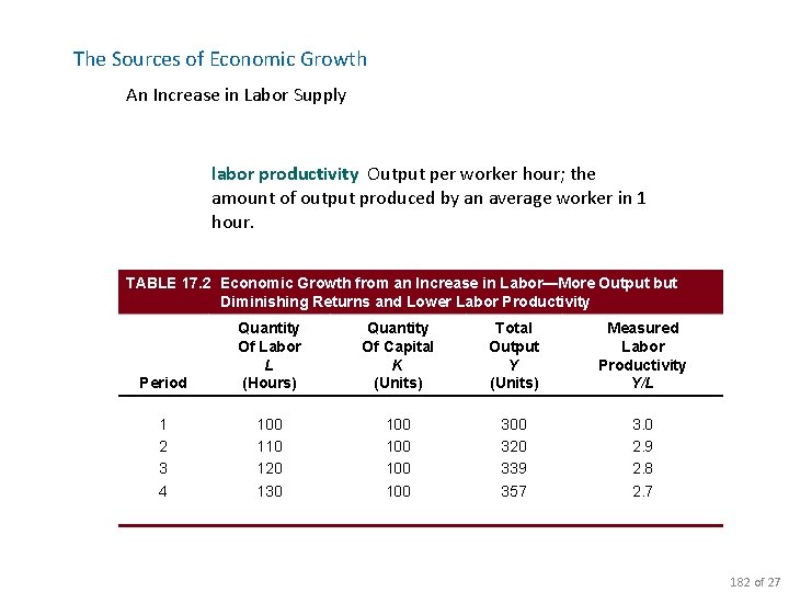
The Sources of Economic Growth An Increase in Labor Supply labor productivity Output per worker hour; the amount of output produced by an average worker in 1 hour. TABLE 17. 2 Economic Growth from an Increase in Labor—More Output but Diminishing Returns and Lower Labor Productivity Period Quantity Of Labor L (Hours) Quantity Of Capital K (Units) Total Output Y (Units) Measured Labor Productivity Y/L 1 2 3 4 100 110 120 130 100 100 300 320 339 357 3. 0 2. 9 2. 8 2. 7 182 of 27

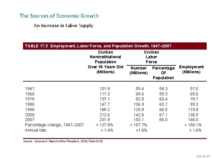
The Sources of Economic Growth An Increase in Labor Supply TABLE 17. 3 Employment, Labor Force, and Population Growth, 1947– 2007 Civilian Noninstitutional Labor Population Force Over 16 Years Old Number Percentage (Millions) Of Population 1947 1960 1970 1980 1990 2007 Percentage change, 1947– 2007 Annual rate 101. 8 117. 3 137. 1 167. 7 189. 2 212. 6 231. 9 + 127. 8% + 1. 4% 59. 4 69. 6 82. 8 106. 9 125. 8 142. 6 153. 1 + 157. 7% +1. 6% 58. 3 59. 3 60. 4 63. 7 66. 5 67. 1 66. 0 Employment (Millions) 57. 0 65. 8 78. 7 99. 3 118. 8 136. 9 146. 0 + 156. 1% + 1. 6% Source: Economic Report of the President, 2008, Table B-35. 183 of 27

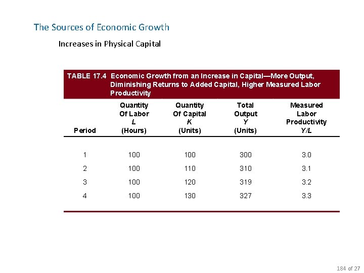
The Sources of Economic Growth Increases in Physical Capital TABLE 17. 4 Economic Growth from an Increase in Capital—More Output, Diminishing Returns to Added Capital, Higher Measured Labor Productivity Period Quantity Of Labor L (Hours) Quantity Of Capital K (Units) Total Output Y (Units) Measured Labor Productivity Y/L 1 100 300 3. 0 2 100 110 3. 1 3 100 120 319 3. 2 4 100 130 327 3. 3 184 of 27

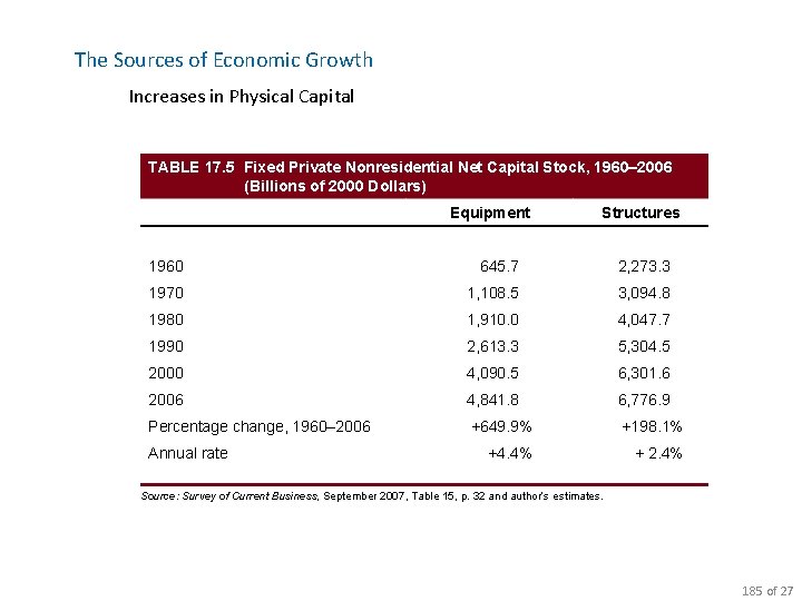
The Sources of Economic Growth Increases in Physical Capital TABLE 17. 5 Fixed Private Nonresidential Net Capital Stock, 1960– 2006 (Billions of 2000 Dollars) Equipment Structures 1960 645. 7 2, 273. 3 1970 1, 108. 5 3, 094. 8 1980 1, 910. 0 4, 047. 7 1990 2, 613. 3 5, 304. 5 2000 4, 090. 5 6, 301. 6 2006 4, 841. 8 6, 776. 9 Percentage change, 1960– 2006 +649. 9% +198. 1% +4. 4% + 2. 4% Annual rate Source: Survey of Current Business, September 2007, Table 15, p. 32 and author’s estimates. 185 of 27

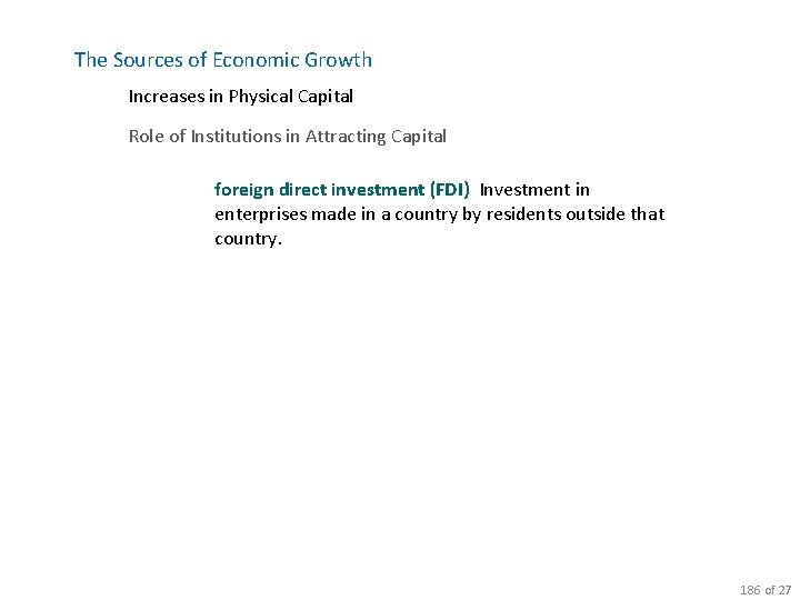
The Sources of Economic Growth Increases in Physical Capital Role of Institutions in Attracting Capital foreign direct investment (FDI) Investment in enterprises made in a country by residents outside that country. 186 of 27

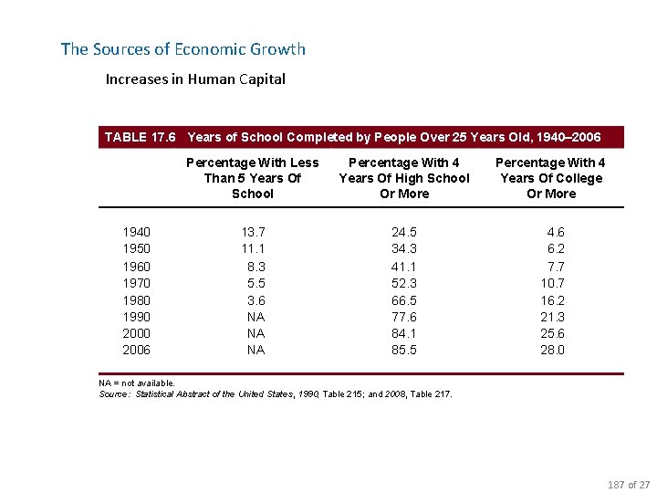
The Sources of Economic Growth Increases in Human Capital TABLE 17. 6 Years of School Completed by People Over 25 Years Old, 1940– 2006 1940 1950 1960 1970 1980 1990 2006 Percentage With Less Than 5 Years Of School Percentage With 4 Years Of High School Or More Percentage With 4 Years Of College Or More 13. 7 11. 1 8. 3 5. 5 3. 6 NA NA NA 24. 5 34. 3 41. 1 52. 3 66. 5 77. 6 84. 1 85. 5 4. 6 6. 2 7. 7 10. 7 16. 2 21. 3 25. 6 28. 0 NA = not available. Source: Statistical Abstract of the United States, 1990, Table 215; and 2008, Table 217. 187 of 27

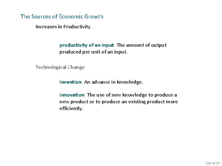
The Sources of Economic Growth Increases in Productivity productivity of an input The amount of output produced per unit of an input. Technological Change invention An advance in knowledge. innovation The use of new knowledge to produce a new product or to produce an existing product more efficiently. 188 of 27

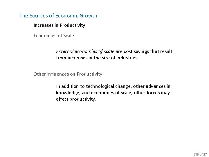
The Sources of Economic Growth Increases in Productivity Economies of Scale External economies of scale are cost savings that result from increases in the size of industries. Other Influences on Productivity In addition to technological change, other advances in knowledge, and economies of scale, other forces may affect productivity. 189 of 27

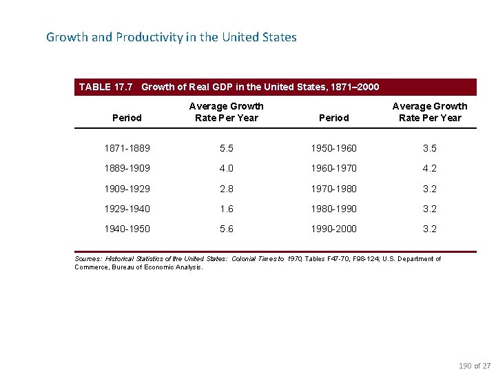
Growth and Productivity in the United States TABLE 17. 7 Growth of Real GDP in the United States, 1871– 2000 Period Average Growth Rate Per Year 1871 -1889 5. 5 1950 -1960 3. 5 1889 -1909 4. 0 1960 -1970 4. 2 1909 -1929 2. 8 1970 -1980 3. 2 1929 -1940 1. 6 1980 -1990 3. 2 1940 -1950 5. 6 1990 -2000 3. 2 Sources: Historical Statistics of the United States: Colonial Times to 1970, Tables F 47 -70, F 98 -124; U. S. Department of Commerce, Bureau of Economic Analysis. 190 of 27

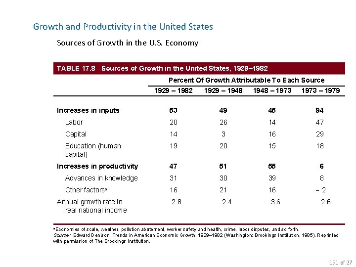
Growth and Productivity in the United States Sources of Growth in the U. S. Economy TABLE 17. 8 Sources of Growth in the United States, 1929– 1982 Percent Of Growth Attributable To Each Source 1929 – 1982 1929 – 1948 – 1973 – 1979 Increases in inputs 53 49 45 94 Labor 20 26 14 47 Capital 14 3 16 29 Education (human capital) 19 20 15 18 Increases in productivity 47 51 55 6 Advances in knowledge 31 30 39 8 Other factorsa 16 21 16 -2 Annual growth rate in real national income 2. 8 2. 4 3. 6 2. 6 a. Economies of scale, weather, pollution abatement, worker safety and health, crime, labor disputes, and so forth. Source: Edward Denison, Trends in American Economic Growth, 1929– 1982 (Washington: Brookings Institution, 1985). Reprinted with permission of The Brookings Institution. 191 of 27

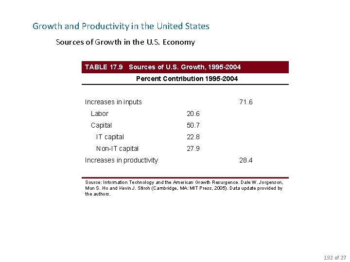
Growth and Productivity in the United States Sources of Growth in the U. S. Economy TABLE 17. 9 Sources of U. S. Growth, 1995 -2004 Percent Contribution 1995 -2004 Increases in inputs 71. 6 Labor 20. 6 Capital 50. 7 IT capital 22. 8 Non-IT capital 27. 9 Increases in productivity 28. 4 Source: Information Technology and the American Growth Resurgence. Dale W. Jorgenson, Mun S. Ho and Kevin J. Stiroh (Cambridge, MA: MIT Press, 2005). Data update provided by the authors. 192 of 27

Economic Growth and Public Policy in the United States Suggested Public Policies to Improve the Quality of Education Policies to Increase the Saving Rate Policies to Stimulate Investment Policies to Increase Research and Development Industrial Policy Can We Really Measure Productivity Changes? One of the leading experts on technology and productivity estimates that we have reasonably good measures of output and productivity in only about 31 percent of the U. S. economy. 193 of 27

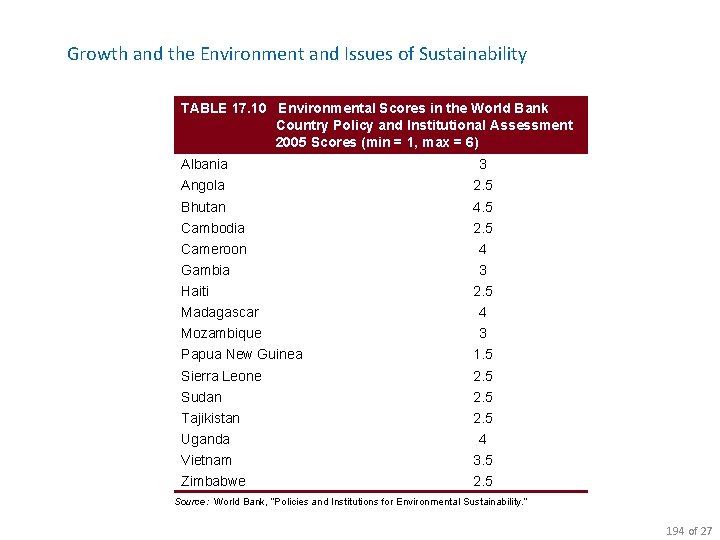
Growth and the Environment and Issues of Sustainability TABLE 17. 10 Environmental Scores in the World Bank Country Policy and Institutional Assessment 2005 Scores (min = 1, max = 6) Albania 3 Angola 2. 5 Bhutan 4. 5 Cambodia 2. 5 Cameroon 4 Gambia 3 Haiti 2. 5 Madagascar 4 Mozambique 3 Papua New Guinea 1. 5 Sierra Leone 2. 5 Sudan 2. 5 Tajikistan 2. 5 Uganda 4 Vietnam 3. 5 Zimbabwe 2. 5 Source: World Bank, “Policies and Institutions for Environmental Sustainability. ” 194 of 27

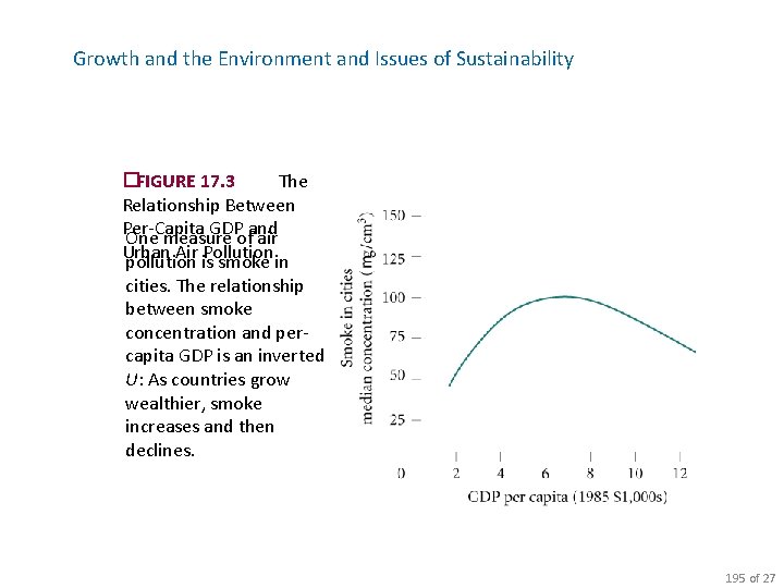
Growth and the Environment and Issues of Sustainability �FIGURE 17. 3 The Relationship Between Per-Capita GDP and One measure of air Urban Air Pollution pollution is smoke in cities. The relationship between smoke concentration and percapita GDP is an inverted U: As countries grow wealthier, smoke increases and then declines. 195 of 27

Growth and the Environment and Issues of Sustainability of Resource Extraction Growth Strategies Much of Southeast Asia has fueled its growth through export-led manufacturing. For countries that have based their growth on resource extraction, there is another set of potential sustainability issues. Because extraction can be accomplished without a well -educated labor force, while other forms of development are more dependent on a skilled- labor base, public investment in infrastructure is especially important. 196 of 27