PARKIN MACROECONOMICS Thirteenth Edition Global Edition 13 FISCAL

PARKIN MACROECONOMICS Thirteenth Edition, Global Edition

13 FISCAL POLICY

After studying this chapter, you will be able to: u Describe the federal budget process and the recent history of outlays, receipts, deficits, and debt u Explain the effects of fiscal policy on potential GDP and economic growth u Explain how fiscal policy choices redistribute benefits and burdens across generations u Explain how fiscal stimulus is used to speed recovery from recession © 2019 Pearson Education Ltd.

The Federal Budget The federal budget is the annual statement of the federal government’s outlays and tax revenues. The federal budget has two purposes: 1. To finance federal government programs and activities 2. To achieve macroeconomic objectives Fiscal policy is the use of the federal budget to achieve macroeconomic objectives, such as full employment, sustained economic growth, and price level stability. © 2019 Pearson Education Ltd.

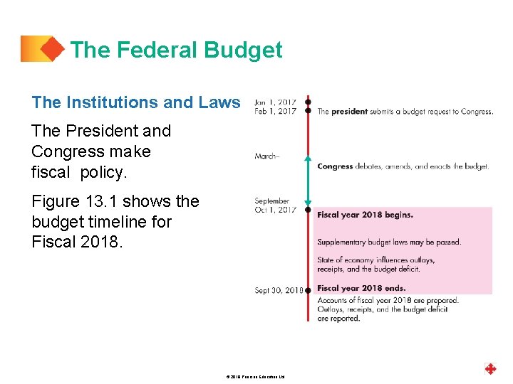
The Federal Budget The Institutions and Laws The President and Congress make fiscal policy.

The Federal Budget Employment Act of 1946 Fiscal policy operates within the framework of the Employment Act of 1946 in which Congress declared that. . . it is the continuing policy and responsibility of the Federal Government to use all practicable means. . . to coordinate and utilize all its plans, functions, and resources. . . to promote maximum employment, production, and purchasing power. © 2019 Pearson Education Ltd.

The Federal Budget The Council of Economic Advisers monitors the economy and keeps the President and the public well informed about the current state of the economy and the best available forecasts of where it is heading. This economic intelligence activity is one source of data that informs the budget-making process. © 2019 Pearson Education Ltd.

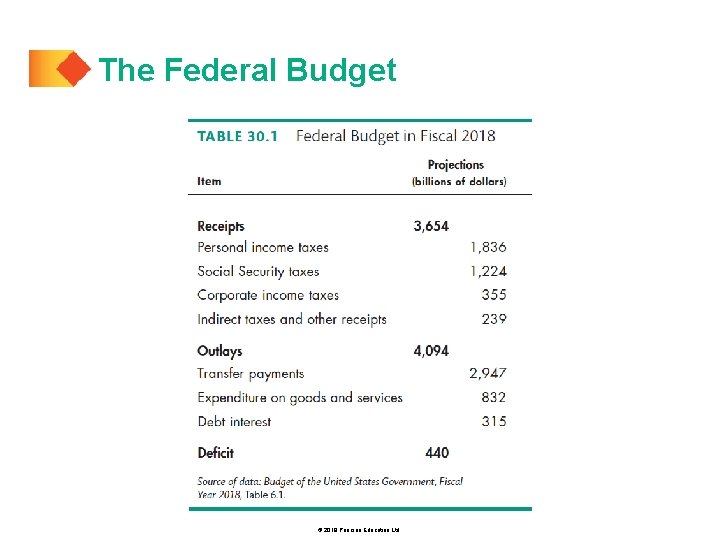
The Federal Budget Highlights of the 2018 Budget The projected fiscal 2018 Federal Budget has receipts of $3, 654 billion, outlays of $4, 094 billion, and a projected deficit of $440 billion. Receipts come from personal income taxes, Social Security taxes, corporate income taxes, and indirect taxes. Personal income taxes are the largest source of receipts. Outlays are transfer payments, expenditure on goods and services, and debt interest. Transfer payments are the largest item of outlays. © 2019 Pearson Education Ltd.

The Federal Budget Surplus or Deficit The federal government’s budget balance equals receipts minus outlays. If receipts exceed outlays, the government has a budget surplus. If outlays exceed receipts, the government has a budget deficit. If receipts equal outlays, the government has a balanced budget. The projected budget deficit in fiscal 2018 is $440 billion. © 2019 Pearson Education Ltd.

The Federal Budget © 2019 Pearson Education Ltd.

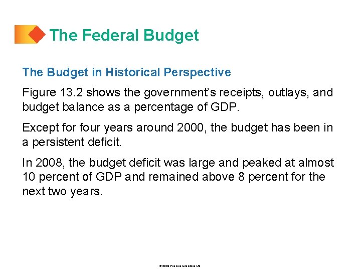
The Federal Budget The Budget in Historical Perspective Figure 13. 2 shows the government’s receipts, outlays, and budget balance as a percentage of GDP. Except for four years around 2000, the budget has been in a persistent deficit. In 2008, the budget deficit was large and peaked at almost 10 percent of GDP and remained above 8 percent for the next two years. © 2019 Pearson Education Ltd.

The Federal Budget Figure 13. 2 shows receipts, outlays, and the budget deficit when

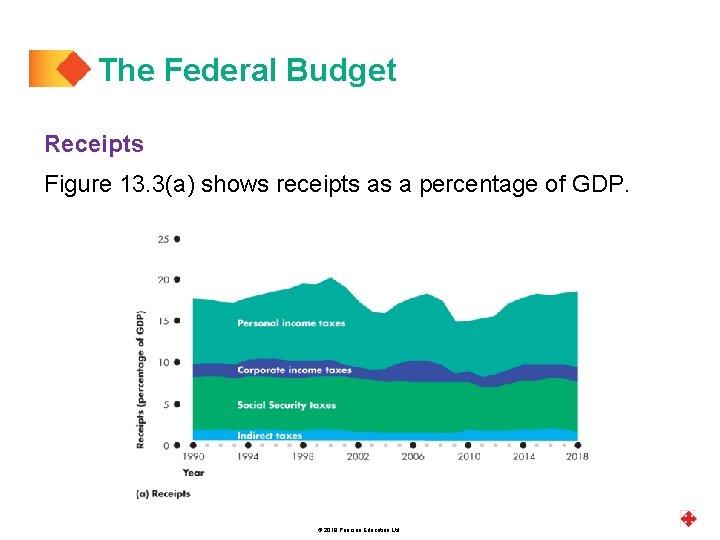
The Federal Budget Receipts Figure 13. 3(a) shows receipts as a percentage of GDP.

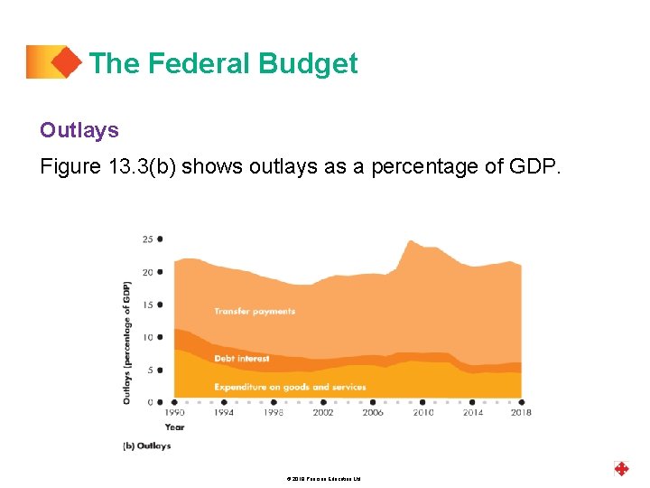
The Federal Budget Outlays Figure 13. 3(b) shows outlays as a percentage of GDP.

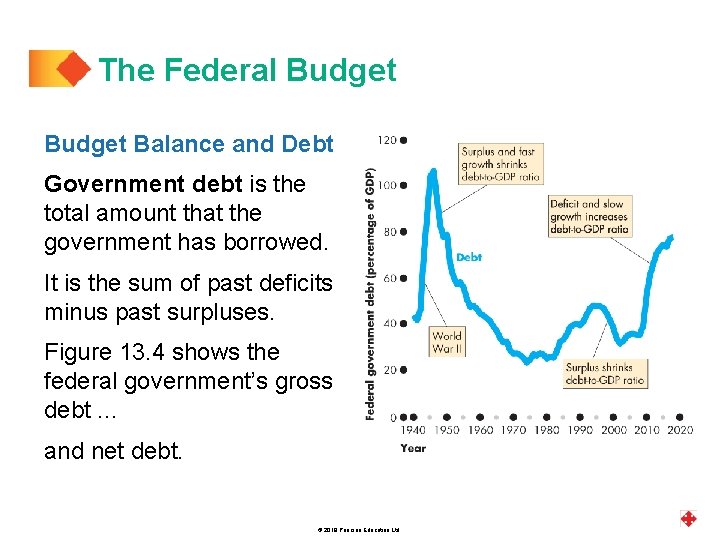
The Federal Budget Balance and Debt Government debt is the total amount that the government has borrowed. It is the sum of past deficits minus past surpluses. Figure 13. 4 shows the federal government’s gross debt. . . and net debt. © 2019 Pearson Education Ltd.

The Federal Budget State and Local Budgets The total government sector includes state and local governments as well as the federal government. In Fiscal 2018, when federal government outlays were about $4, 094 billion, state and local outlays were a further $3, 600 billion. Most of state expenditures were on public schools, colleges, and universities ($1, 400 billion); local police and fire services; and roads. © 2019 Pearson Education Ltd.

Supply-Side Effects of Fiscal Policy Fiscal policy has important effects on employment, potential GDP, and aggregate supply—called supply-side effects. An income tax changes full employment and potential GDP. © 2019 Pearson Education Ltd.

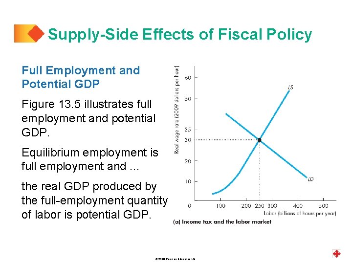
Supply-Side Effects of Fiscal Policy Full Employment and Potential GDP Figure 13. 5 illustrates full employment and potential GDP. Equilibrium employment is full employment and. . . the real GDP produced by the full-employment quantity of labor is potential GDP. © 2019 Pearson Education Ltd.

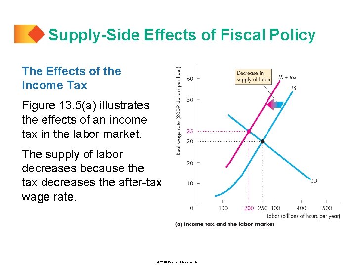
Supply-Side Effects of Fiscal Policy The Effects of the Income Tax Figure 13. 5(a) illustrates the effects of an income tax in the labor market. The supply of labor decreases because the tax decreases the after-tax wage rate. © 2019 Pearson Education Ltd.

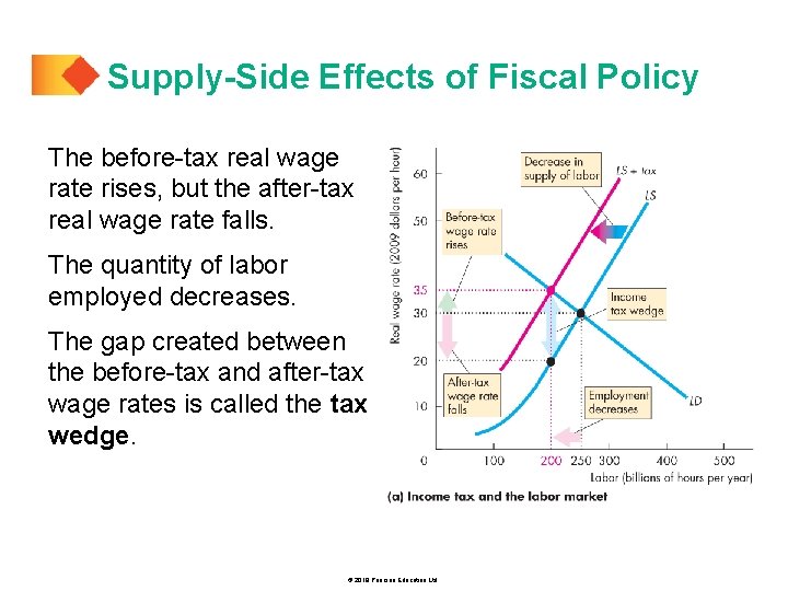
Supply-Side Effects of Fiscal Policy The before-tax real wage rate rises, but the after-tax real wage rate falls. The quantity of labor employed decreases. The gap created between the before-tax and after-tax wage rates is called the tax wedge. © 2019 Pearson Education Ltd.

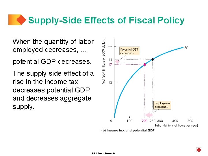
Supply-Side Effects of Fiscal Policy When the quantity of labor employed decreases, … potential GDP decreases. The supply-side effect of a rise in the income tax decreases potential GDP and decreases aggregate supply. © 2019 Pearson Education Ltd.

Supply-Side Effects of Fiscal Policy Taxes on Expenditure and the Tax Wedge Taxes on consumption expenditure add to the tax wedge. The reason is that a tax on consumption raises the prices paid for consumption goods and services and is equivalent to a cut in the real wage rate. If the income tax rate is 25 percent and the tax rate on consumption expenditure is 10 percent, a dollar earned buys only 65 cents worth of goods and services. The tax wedge is 35 percent. © 2019 Pearson Education Ltd.

Supply-Side Effects of Fiscal Policy Taxes and the Incentive to Save and Invest A tax on capital income lowers the quantity of saving and investment and slows the growth rate of real GDP. The interest rate that influences saving and investment is the real after-tax interest rate. The real after-tax interest rate subtracts the income tax paid on interest income from the real interest. Taxes depend on the nominal interest rate. So the true tax on interest income depends on the inflation rate. © 2019 Pearson Education Ltd.

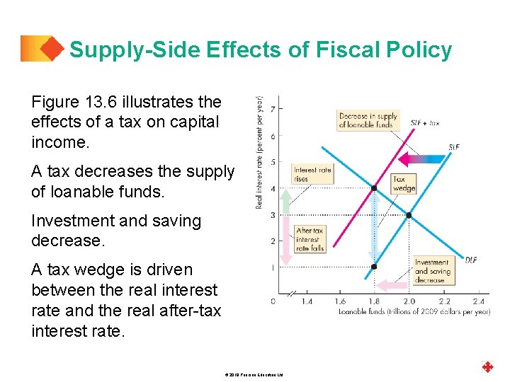
Supply-Side Effects of Fiscal Policy Figure 13. 6 illustrates the effects of a tax on capital income. A tax decreases the supply of loanable funds. Investment and saving decrease. A tax wedge is driven between the real interest rate and the real after-tax interest rate. © 2019 Pearson Education Ltd.

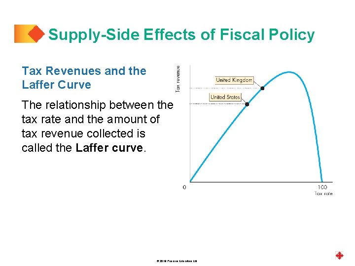
Supply-Side Effects of Fiscal Policy Tax Revenues and the Laffer Curve The relationship between the tax rate and the amount of tax revenue collected is called the Laffer curve. © 2019 Pearson Education Ltd.

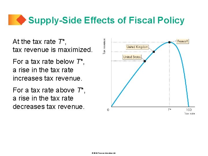
Supply-Side Effects of Fiscal Policy At the tax rate T*, tax revenue is maximized. For a tax rate below T*, a rise in the tax rate increases tax revenue. For a tax rate above T*, a rise in the tax rate decreases tax revenue. © 2019 Pearson Education Ltd.

Generational Effects of Fiscal Policy Is the budget deficit a burden on future generations? Is the budget deficit the only burden on future generations? What about the deficit in the Social Security fund? Does it matter who owns the bonds that the government sells to finance its deficit? To answer questions like these, we use a tool called generational accounting. Generational accounting is an accounting system that measures the lifetime tax burden and benefits of each generation. © 2019 Pearson Education Ltd.

Generational Effects of Fiscal Policy Generational Accounting and Present Value Taxes are paid by people with jobs. Social Security benefits are paid to people after they retire. So to compare the value of an amount of money at one date (working years) with that at a later date (retirement years), we use the concept of present value. A present value is an amount of money that, if invested today, will grow to equal a given future amount when the interest that it earns is taken into account. © 2019 Pearson Education Ltd.

Generational Effects of Fiscal Policy For example: If the interest rate is 5 percent a year, $1, 000 invested today will grow, with interest, to $11, 467 after 50 years. The present value (2018) of $11, 467 in 2068 is $1, 000. © 2019 Pearson Education Ltd.

Generational Effects of Fiscal Policy The Social Security Time Bomb Using generational accounting and present values, economists have found that the federal government is facing a Social Security time bomb! In 2008, the first of the baby boomers started collecting Social Security pensions and in 2011, they became eligible for Medicare benefits. By 2030, all the baby boomers will have reached retirement age and the population supported by Social Security will have doubled. © 2019 Pearson Education Ltd.

Generational Effects of Fiscal Policy Under the existing Social Security laws, the federal government has an obligation to pay pensions and Medicare benefits on an already declared scale. To assess the full extent of the government’s obligations, economists use the concept of fiscal imbalance. Fiscal imbalance is the present value of the government’s commitments to pay benefits minus the present value of its tax revenues. Gokhale and Smetters estimated that the fiscal imbalance was $68 trillion in 2014— 4 times the value of total production in 2014 ($17 trillion). © 2019 Pearson Education Ltd.

Generational Effects of Fiscal Policy How can the government meet its Social security obligations? Gokhale and Smetters consider four alternatives: 1. Taxes 2. Raise income se Social Security taxes 3. Cut Social Security benefits 4. Cut federal government discretionary spending Starting in 2003, income taxes would need to be raised by 69 percent, or Social Security taxes raised by 95 percent, or Social Security benefits cut by 56 percent. © 2019 Pearson Education Ltd.

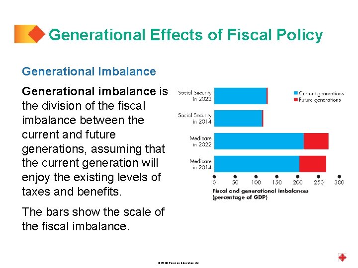
Generational Effects of Fiscal Policy Generational Imbalance Generational imbalance is the division of the fiscal imbalance between the current and future generations, assuming that the current generation will enjoy the existing levels of taxes and benefits. The bars show the scale of the fiscal imbalance. © 2019 Pearson Education Ltd.

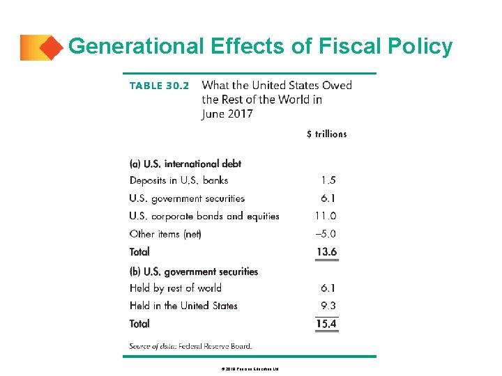
Generational Effects of Fiscal Policy International Debt How much investment have we paid for by borrowing from the rest of the world? And how much U. S. government debt is held abroad? In June 2017, the United States had a net debt to the rest of the world of $13. 6 trillion. Of that debt, $6. 1 trillion was U. S. government debt. U. S. corporations used $11. 0 trillion of foreign funds. © 2019 Pearson Education Ltd.

Generational Effects of Fiscal Policy © 2019 Pearson Education Ltd.

Fiscal Stimulus A fiscal stimulus is the use of fiscal policy to increase production and employment. Fiscal stimulus can be either § Automatic § Discretionary Automatic fiscal policy is a fiscal policy action triggered by the state of the economy with no government action. Discretionary fiscal policy is a policy action that is initiated by an act of Congress. © 2019 Pearson Education Ltd.

Fiscal Stimulus Automatic Fiscal Policy and Cyclical and Structural Budget Balances Two items in the government budget change automatically in response to the state of the economy. § Tax revenues § Needs-tested spending © 2019 Pearson Education Ltd.

Fiscal Stimulus Automatic Changes in Tax Revenues Congress sets the tax rates that people must pay. The tax dollars people pay depend on tax rates and incomes. But incomes vary with real GDP, so tax revenues depend on real GDP. When real GDP increases in an expansion, tax revenues increase. When real GDP decreases in a recession, tax revenues decrease. © 2019 Pearson Education Ltd.

Fiscal Stimulus Needs-Tested Spending The government creates programs that pay benefits to qualified people and businesses. These transfer payments depend on the economic state of the economy. When the economy is in an expansion, unemployment falls, so needs-tested spending decreases. When the economy is in a recession, unemployment rises, so needs-tested spending increases. © 2019 Pearson Education Ltd.

Fiscal Stimulus Automatic Stimulus In a recession, receipts decrease and outlays increase. So the budget provides an automatic stimulus that helps shrink the recessionary gap. In a boom, receipts increase and outlays decrease. So the budget provides automatic restraint that helps shrink the inflationary gap. © 2019 Pearson Education Ltd.

Fiscal Stimulus Cyclical and Structural Balances The structural surplus or deficit is the budget balance that would occur if the economy were at full employment and real GDP were equal to potential GDP. The cyclical surplus or deficit is the actual surplus or deficit minus the structural surplus or deficit. That is, a cyclical surplus or deficit is the surplus or deficit that occurs purely because real GDP does not equal potential GDP. © 2019 Pearson Education Ltd.

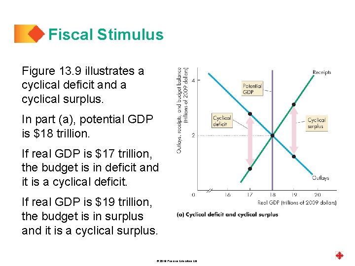
Fiscal Stimulus Figure 13. 9 illustrates a cyclical deficit and a cyclical surplus. In part (a), potential GDP is $18 trillion. If real GDP is $17 trillion, the budget is in deficit and it is a cyclical deficit. If real GDP is $19 trillion, the budget is in surplus and it is a cyclical surplus. © 2019 Pearson Education Ltd.

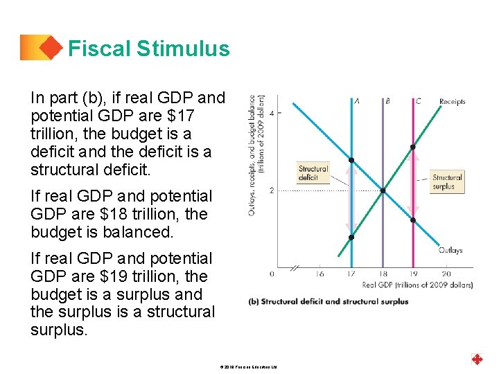
Fiscal Stimulus In part (b), if real GDP and potential GDP are $17 trillion, the budget is a deficit and the deficit is a structural deficit. If real GDP and potential GDP are $18 trillion, the budget is balanced. If real GDP and potential GDP are $19 trillion, the budget is a surplus and the surplus is a structural surplus. © 2019 Pearson Education Ltd.

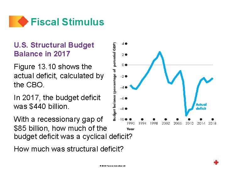
Fiscal Stimulus U. S. Structural Budget Balance in 2017 Figure 13. 10 shows the actual deficit, calculated by the CBO. In 2017, the budget deficit was $440 billion. With a recessionary gap of $85 billion, how much of the budget deficit was a cyclical deficit? How much was structural deficit? © 2019 Pearson Education Ltd.

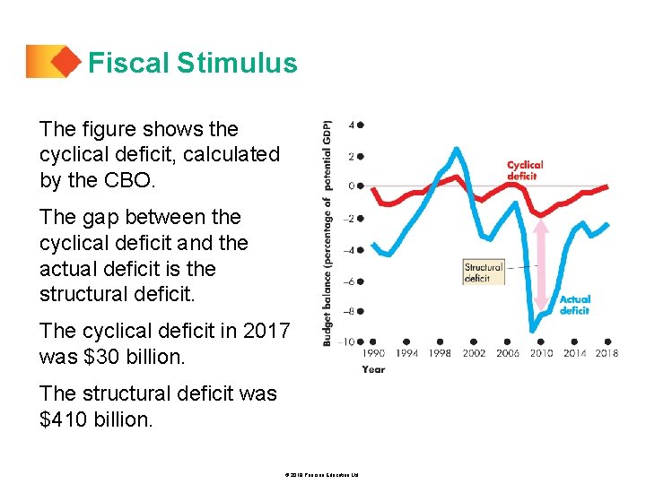
Fiscal Stimulus The figure shows the cyclical deficit, calculated by the CBO. The gap between the cyclical deficit and the actual deficit is the structural deficit. The cyclical deficit in 2017 was $30 billion. The structural deficit was $410 billion. © 2019 Pearson Education Ltd.

Fiscal Stimulus Discretionary Fiscal Stimulus Most discretionary fiscal stimulus focuses on its effects on aggregate demand. Fiscal Stimulus and Aggregate Demand Changes in government expenditure and taxes change aggregate demand have multiplier effects. Two main fiscal multipliers are § Government expenditure multiplier § Tax multiplier © 2019 Pearson Education Ltd.

Fiscal Stimulus The government expenditure multiplier is the quantitative effect of a change in government expenditure on real GDP. Because government expenditure is a component of aggregate expenditure, an increase in government expenditure increases real GDP. When real GDP increases, incomes rise and consumption expenditure increases. Aggregate demand increases. If this were the only consequence of the increase in government expenditure, the multiplier would be >1. © 2019 Pearson Education Ltd.

Fiscal Stimulus But an increase in government expenditure increases government borrowing and raises the real interest rate. With the higher cost of borrowing, investment decreases, which partly offsets the increase in government expenditure. If this were the only consequence of the increase in government expenditure, the multiplier would be < 1. Which effect is stronger? The consensus is that the crowding-out effect dominates and the multiplier is <1. © 2019 Pearson Education Ltd.

Fiscal Stimulus The tax multiplier is the quantitative effect of a change in taxes on aggregate demand. The demand-side effects of a tax cut are likely to be smaller than an equivalent increase in government expenditure. © 2019 Pearson Education Ltd.

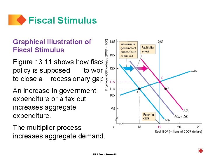
Fiscal Stimulus Graphical Illustration of Fiscal Stimulus Figure 13. 11 shows how fiscal policy is supposed to work to close a recessionary gap. An increase in government expenditure or a tax cut increases aggregate expenditure. The multiplier process increases aggregate demand. © 2019 Pearson Education Ltd.

Fiscal Stimulus and Aggregate Supply Taxes drive a wedge between the cost of labor and the take-home pay and between the cost of borrowing and the return on lending. Taxes decrease employment, saving, and investment and decrease real GDP and its growth rate. A tax cut decreases these negative effects and increases real GDP and its growth rate. The supply-side effects of a tax cut probably dominate the demand-side effects and make the tax multiplier larger than the government expenditure multiplier. © 2019 Pearson Education Ltd.

Fiscal Stimulus Magnitude of Stimulus Economists have diverging views about the size of the fiscal multipliers because there is insufficient empirical evidence on which to pin their size with accuracy. This fact makes it impossible for Congress to determine the amount of stimulus needed to close a given output gap. Also, the actual output gap is not known and can only be estimated with error. So discretionary fiscal policy is risky. © 2019 Pearson Education Ltd.

Fiscal Stimulus Time Lags The use of discretionary fiscal policy is also seriously hampered by three time lags: § Recognition lag—the time it takes to figure out that fiscal policy action is needed. § Law-making lag—the time it takes Congress to pass the laws needed to change taxes or spending. § Impact lag—the time it takes from passing a tax or spending change to its effect on real GDP being felt. © 2019 Pearson Education Ltd.