Macroeconomics LECTURE SLIDES SET 3 Professor Antonio Ciccone

Macroeconomics LECTURE SLIDES SET 3 Professor Antonio Ciccone Macroeconomics SLIDE SET 3 Slide 1

II. ECONOMIC GROWTH WITH ENDOGENOUS SAVINGS Macroeconomics SLIDE SET 3 Slide 2

1. Household savings behavior Macroeconomics SLIDE SET 3 Slide 3

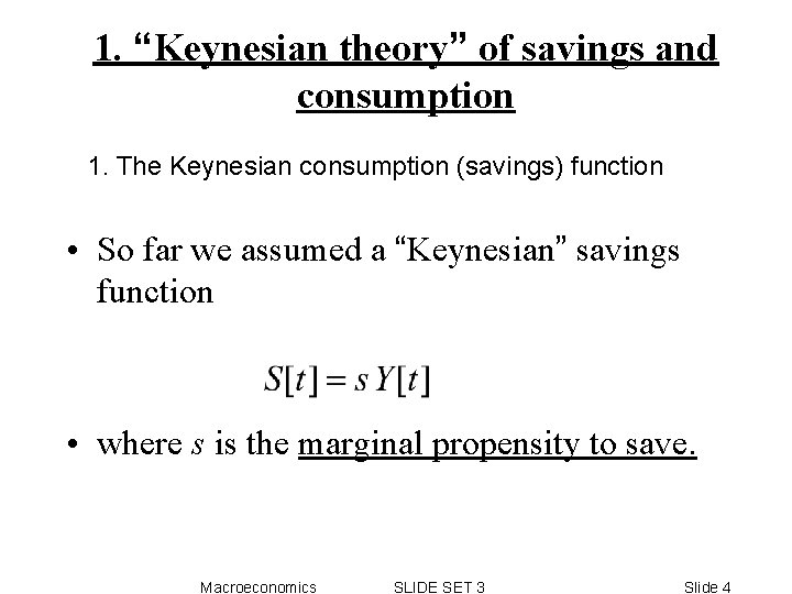
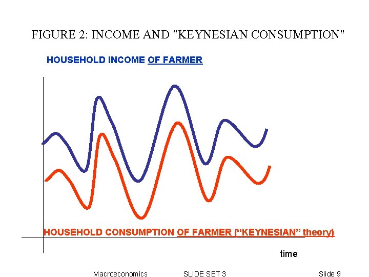
1. “Keynesian theory” of savings and consumption 1. The Keynesian consumption (savings) function • So far we assumed a “Keynesian” savings function • where s is the marginal propensity to save. Macroeconomics SLIDE SET 3 Slide 4

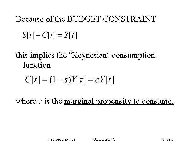
Because of the BUDGET CONSTRAINT this implies the “Keynesian” consumption function where c is the marginal propensity to consume. Macroeconomics SLIDE SET 3 Slide 5

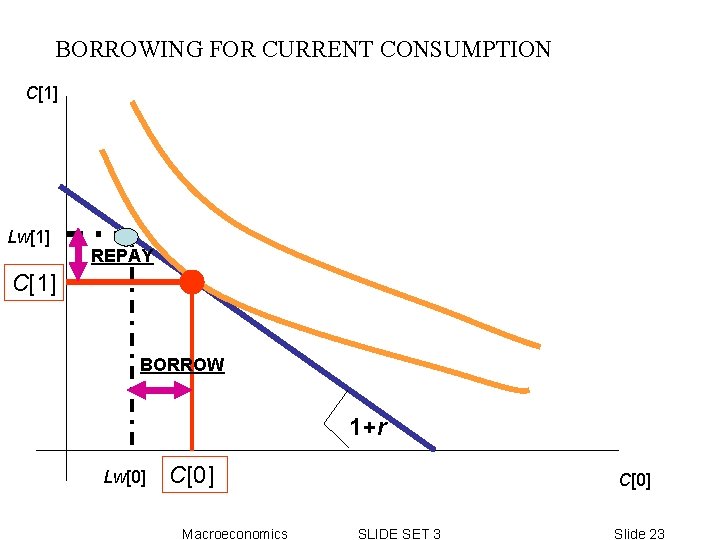
2. Limitations CONCEPTUAL The consumption behavior is assumed to be “mechanic” and “shortsighted”: – Are households really only looking at CURRENT income when deciding consumption? Not really. Many households borrow from banks in order to be able to consume more today because they know they will be able to pay the money back in the future. – If people save, presumably they are doing this for future consumption. Hence, savings is a FORWARD-LOOKING decision and must take into account what happens in the future. Macroeconomics SLIDE SET 3 Slide 6

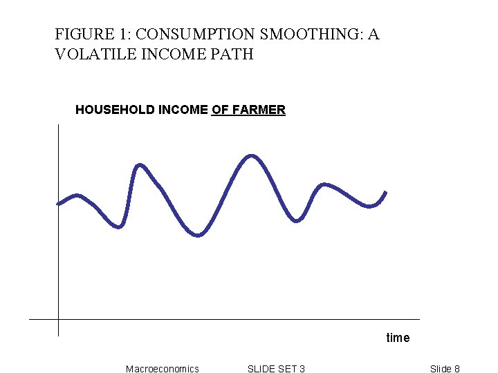
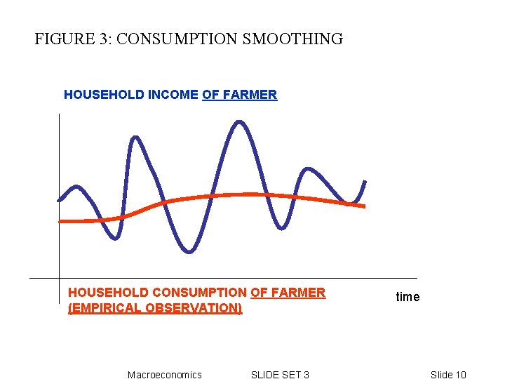
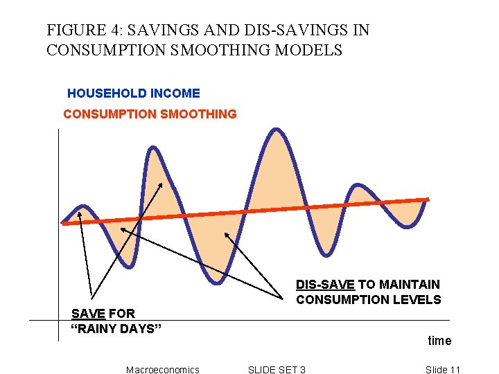
Assuming savings as a function of current income therefore appears to contradict the use that households make of their savings. EMPIRICAL “Consumption smoothing: ” – Empirically, we observe that households smooth consumption. To put it differently, the income of households is often more volatile than their consumption. This suggests that households look forward and try to stabilize consumption (their standard of living) as much as they can. Macroeconomics SLIDE SET 3 Slide 7

FIGURE 1: CONSUMPTION SMOOTHING: A VOLATILE INCOME PATH HOUSEHOLD INCOME OF FARMER time Macroeconomics SLIDE SET 3 Slide 8

FIGURE 2: INCOME AND "KEYNESIAN CONSUMPTION" HOUSEHOLD INCOME OF FARMER HOUSEHOLD CONSUMPTION OF FARMER (“KEYNESIAN” theory) time Macroeconomics SLIDE SET 3 Slide 9

FIGURE 3: CONSUMPTION SMOOTHING HOUSEHOLD INCOME OF FARMER HOUSEHOLD CONSUMPTION OF FARMER (EMPIRICAL OBSERVATION) Macroeconomics SLIDE SET 3 time Slide 10

FIGURE 4: SAVINGS AND DIS-SAVINGS IN CONSUMPTION SMOOTHING MODELS HOUSEHOLD INCOME CONSUMPTION SMOOTHING DIS-SAVE TO MAINTAIN CONSUMPTION LEVELS SAVE FOR “RAINY DAYS” Macroeconomics time SLIDE SET 3 Slide 11

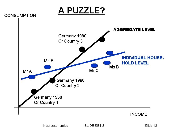
INTERESTINGLY: The Keynesian theory of consumption seems to do better at the aggregate level than at the level of individual households. For example: – Keynesian theory does well in describing relationship between consumption and income of a country at different in different years – Theory does also well in describing relationship between consumption and income across different countries Macroeconomics SLIDE SET 3 Slide 12

A PUZZLE? CONSUMPTION AGGREGATE LEVEL Germany 1980 Or Country 3 Ms B Mr C Mr A Ms D INDIVIDUAL HOUSEHOLD LEVEL Germany 1960 Or Country 2 Germany 1950 Or Country 1 INCOME Macroeconomics SLIDE SET 3 Slide 13

2. The permanent income theory of consumption and savings 1. Basic idea and two-period model Households make consumption decisions: • LOOKING FORWARD to future • USING SAVINGS AND LOANS from BANKS to maintain their living standards STABLE in time to the extent possible Macroeconomics SLIDE SET 3 Slide 14

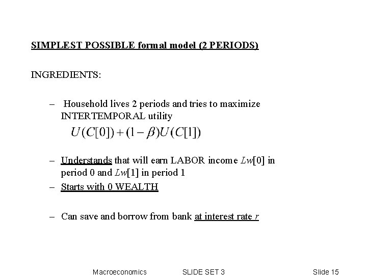
SIMPLEST POSSIBLE formal model (2 PERIODS) INGREDIENTS: – Household lives 2 periods and tries to maximize INTERTEMPORAL utility – Understands that will earn LABOR income Lw[0] in period 0 and Lw[1] in period 1 – Starts with 0 WEALTH – Can save and borrow from bank at interest rate r Macroeconomics SLIDE SET 3 Slide 15

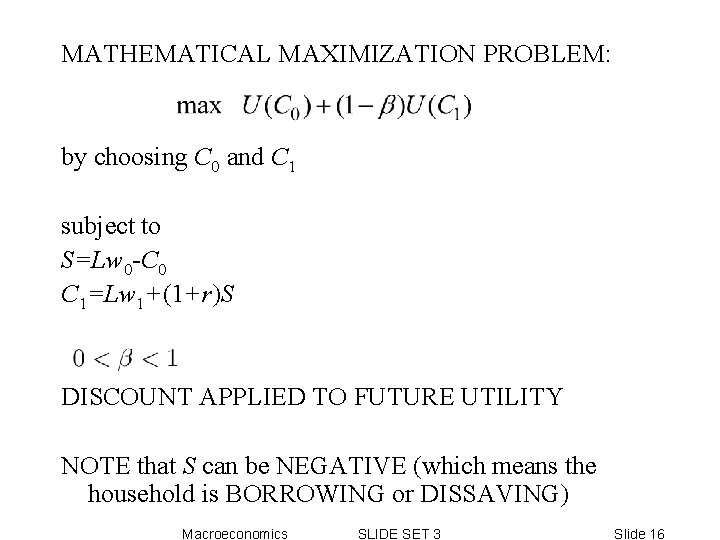
MATHEMATICAL MAXIMIZATION PROBLEM: by choosing C 0 and C 1 subject to S=Lw 0 -C 0 C 1=Lw 1+(1+r)S DISCOUNT APPLIED TO FUTURE UTILITY NOTE that S can be NEGATIVE (which means the household is BORROWING or DISSAVING) Macroeconomics SLIDE SET 3 Slide 16

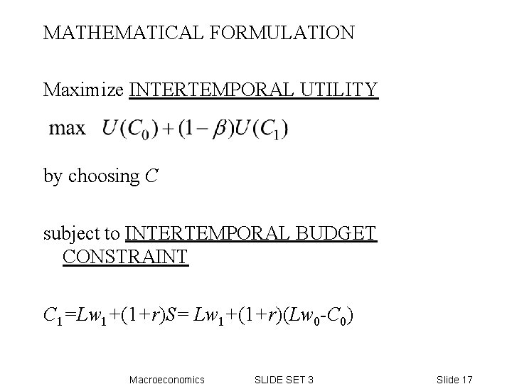
MATHEMATICAL FORMULATION Maximize INTERTEMPORAL UTILITY by choosing C subject to INTERTEMPORAL BUDGET CONSTRAINT C 1=Lw 1+(1+r)S= Lw 1+(1+r)(Lw 0 -C 0) Macroeconomics SLIDE SET 3 Slide 17

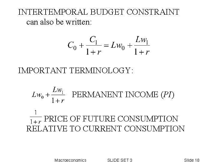
INTERTEMPORAL BUDGET CONSTRAINT can also be written: IMPORTANT TERMINOLOGY: PERMANENT INCOME (PI) PRICE OF FUTURE CONSUMPTION RELATIVE TO CURRENT CONSUMPTION Macroeconomics SLIDE SET 3 Slide 18

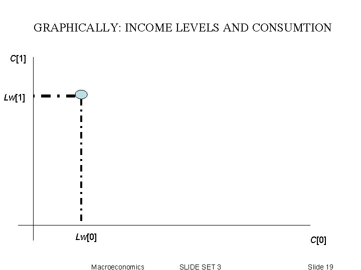
GRAPHICALLY: INCOME LEVELS AND CONSUMTION C[1] Lw[0] Macroeconomics C[0] SLIDE SET 3 Slide 19

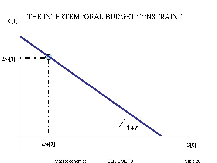
C[1] THE INTERTEMPORAL BUDGET CONSTRAINT Lw[1] 1+r Lw[0] C[0] Macroeconomics SLIDE SET 3 Slide 20

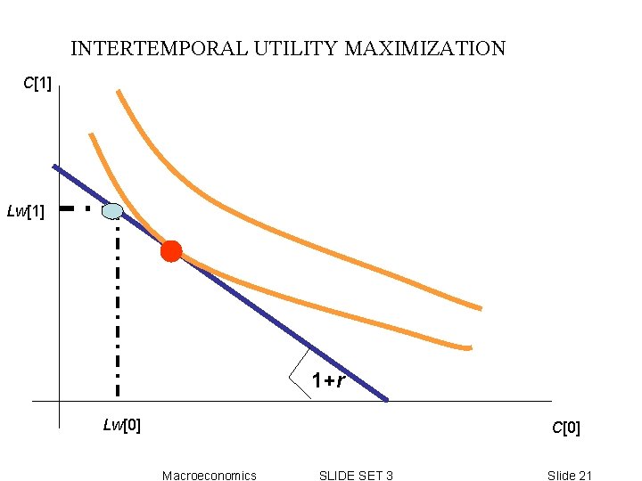
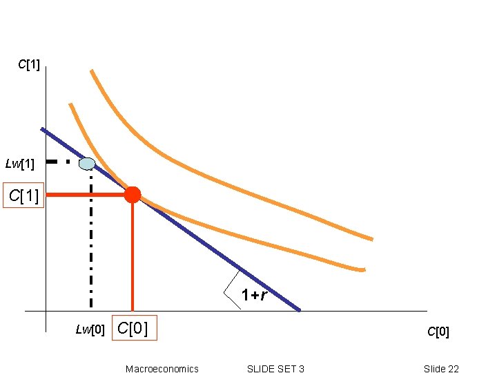
INTERTEMPORAL UTILITY MAXIMIZATION C[1] Lw[1] 1+r Lw[0] C[0] Macroeconomics SLIDE SET 3 Slide 21

C[1] Lw[1] C[1] 1+r Lw[0] C[0] Macroeconomics C[0] SLIDE SET 3 Slide 22

BORROWING FOR CURRENT CONSUMPTION C[1] Lw[1] REPAY C[1] BORROW 1+r Lw[0] C[0] Macroeconomics C[0] SLIDE SET 3 Slide 23

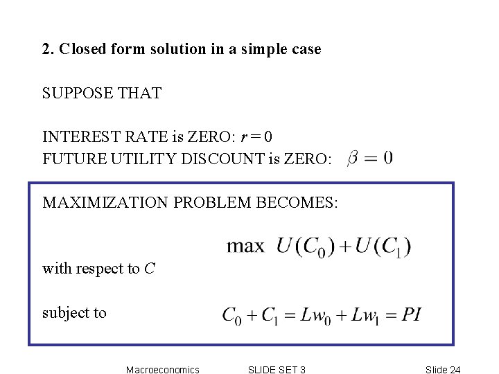
2. Closed form solution in a simple case SUPPOSE THAT INTEREST RATE is ZERO: r = 0 FUTURE UTILITY DISCOUNT is ZERO: MAXIMIZATION PROBLEM BECOMES: with respect to C subject to Macroeconomics SLIDE SET 3 Slide 24

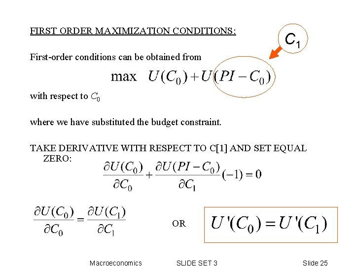
FIRST ORDER MAXIMIZATION CONDITIONS: C 1 First-order conditions can be obtained from with respect to C 0 where we have substituted the budget constraint. TAKE DERIVATIVE WITH RESPECT TO C[1] AND SET EQUAL ZERO: OR Macroeconomics SLIDE SET 3 Slide 25

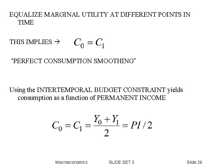
EQUALIZE MARGINAL UTILITY AT DIFFERENT POINTS IN TIME THIS IMPLIES “PERFECT CONSUMPTION SMOOTHING” Using the INTERTEMPORAL BUDGET CONSTRAINT yields consumption as a function of PERMANENT INCOME Macroeconomics SLIDE SET 3 Slide 26

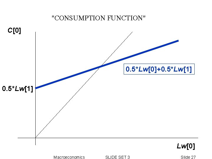
"CONSUMPTION FUNCTION" C[0] 0. 5*Lw[0]+0. 5*Lw[1] Lw[0] Macroeconomics SLIDE SET 3 Slide 27

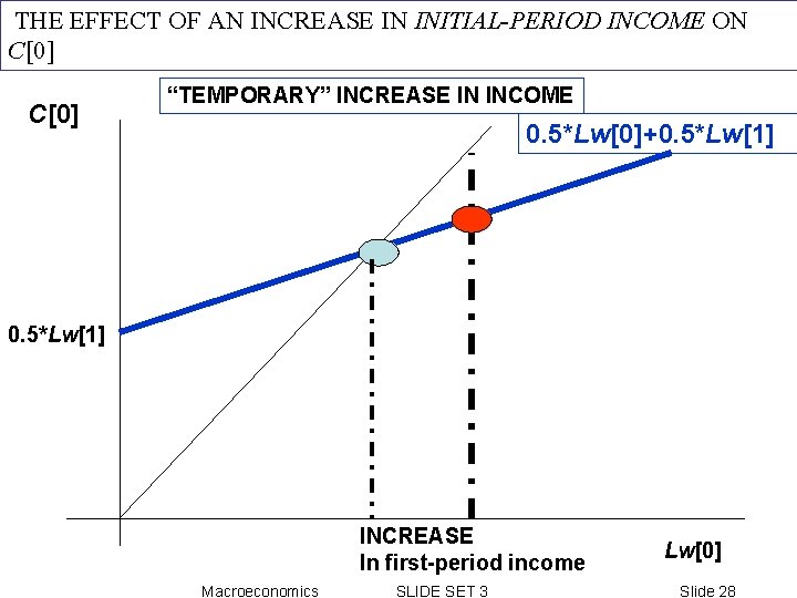
THE EFFECT OF AN INCREASE IN INITIAL-PERIOD INCOME ON C[0] “TEMPORARY” INCREASE IN INCOME 0. 5*Lw[0]+0. 5*Lw[1] INCREASE In first-period income Macroeconomics SLIDE SET 3 Lw[0] Slide 28

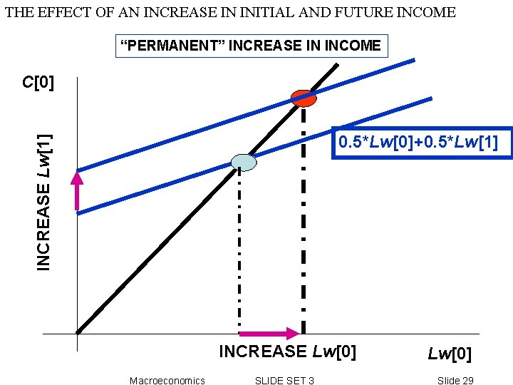
THE EFFECT OF AN INCREASE IN INITIAL AND FUTURE INCOME “PERMANENT” INCREASE IN INCOME C[0] INCREASE Lw[1] 0. 5*Lw[0]+0. 5*Lw[1] INCREASE Lw[0] Macroeconomics SLIDE SET 3 Lw[0] Slide 29

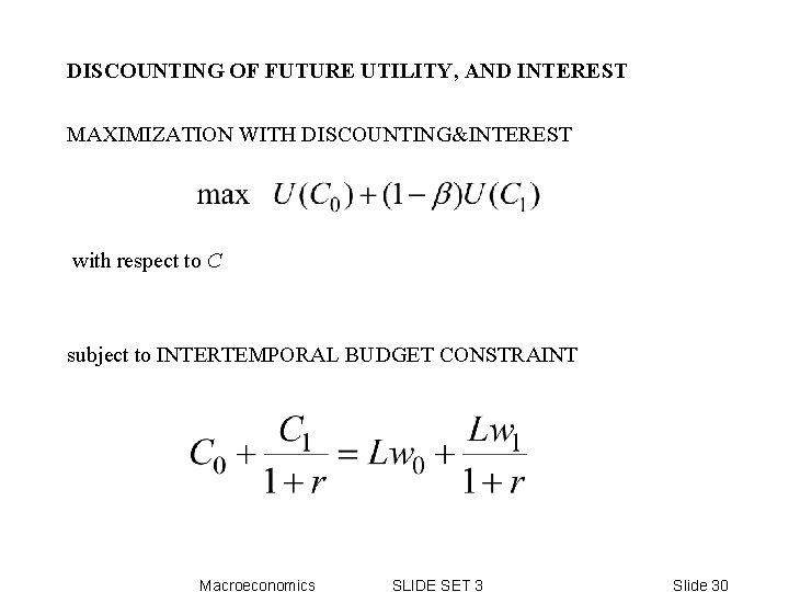
DISCOUNTING OF FUTURE UTILITY, AND INTEREST MAXIMIZATION WITH DISCOUNTING&INTEREST with respect to C subject to INTERTEMPORAL BUDGET CONSTRAINT Macroeconomics SLIDE SET 3 Slide 30

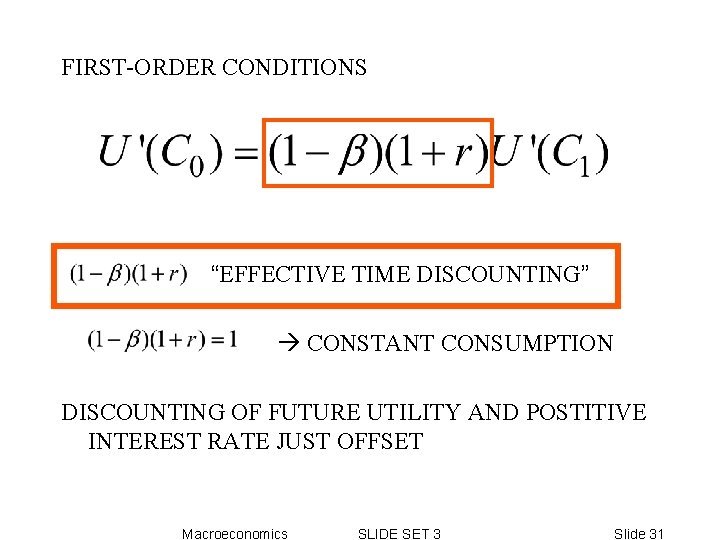
FIRST-ORDER CONDITIONS “EFFECTIVE TIME DISCOUNTING” CONSTANT CONSUMPTION DISCOUNTING OF FUTURE UTILITY AND POSTITIVE INTEREST RATE JUST OFFSET Macroeconomics SLIDE SET 3 Slide 31

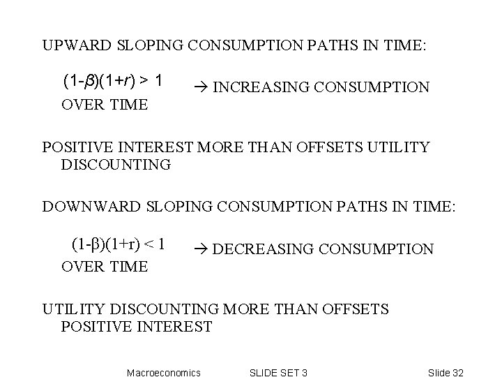
UPWARD SLOPING CONSUMPTION PATHS IN TIME: (1 -β)(1+r) > 1 OVER TIME INCREASING CONSUMPTION POSITIVE INTEREST MORE THAN OFFSETS UTILITY DISCOUNTING DOWNWARD SLOPING CONSUMPTION PATHS IN TIME: (1 -β)(1+r) < 1 OVER TIME DECREASING CONSUMPTION UTILITY DISCOUNTING MORE THAN OFFSETS POSITIVE INTEREST Macroeconomics SLIDE SET 3 Slide 32

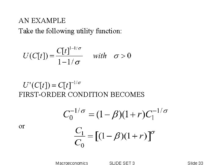
AN EXAMPLE Take the following utility function: FIRST-ORDER CONDITION BECOMES or Macroeconomics SLIDE SET 3 Slide 33

3. The case of 3 and more periods -- Timing -- Intertemporal budget constraint -- Optimality conditions -- Time consistency Macroeconomics SLIDE SET 3 Slide 34

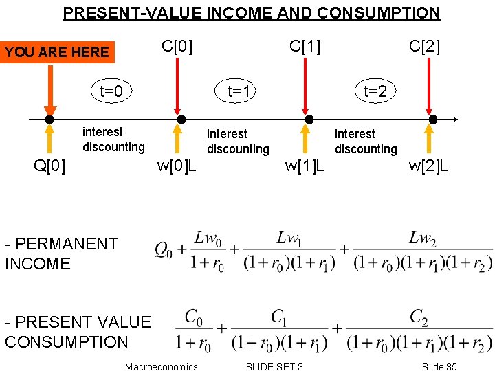
PRESENT-VALUE INCOME AND CONSUMPTION C[0] YOU ARE HERE C[1] t=0 t=1 interest discounting Q[0] w[0]L C[2] t=2 interest discounting w[1]L w[2]L - PERMANENT INCOME - PRESENT VALUE CONSUMPTION Macroeconomics SLIDE SET 3 Slide 35

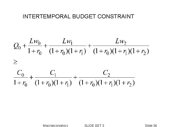
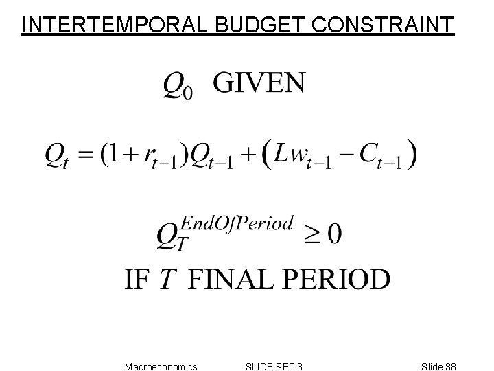
INTERTEMPORAL BUDGET CONSTRAINT Macroeconomics SLIDE SET 3 Slide 36

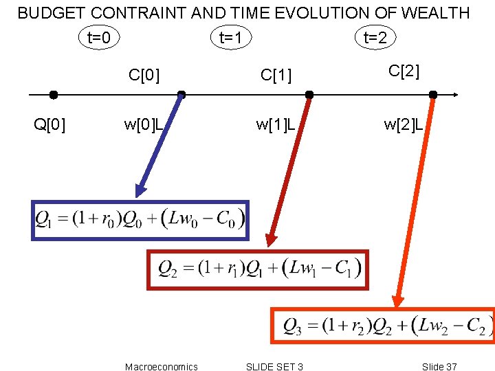
BUDGET CONTRAINT AND TIME EVOLUTION OF WEALTH t=0 t=1 t=2 Q[0] C[1] C[2] w[0]L w[1]L w[2]L Macroeconomics SLIDE SET 3 Slide 37

INTERTEMPORAL BUDGET CONSTRAINT Macroeconomics SLIDE SET 3 Slide 38

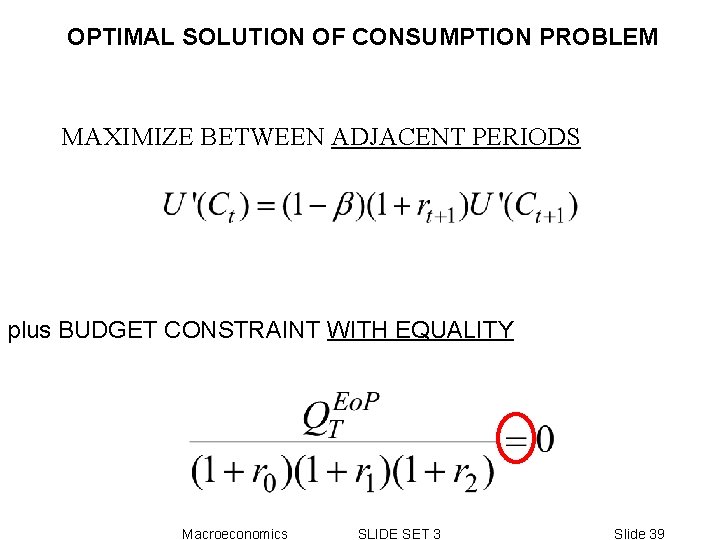
OPTIMAL SOLUTION OF CONSUMPTION PROBLEM MAXIMIZE BETWEEN ADJACENT PERIODS plus BUDGET CONSTRAINT WITH EQUALITY Macroeconomics SLIDE SET 3 Slide 39

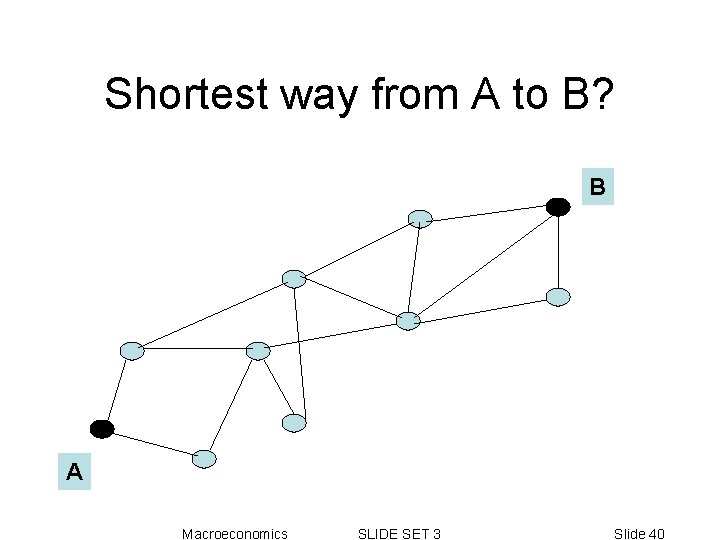
Shortest way from A to B? B A Macroeconomics SLIDE SET 3 Slide 40

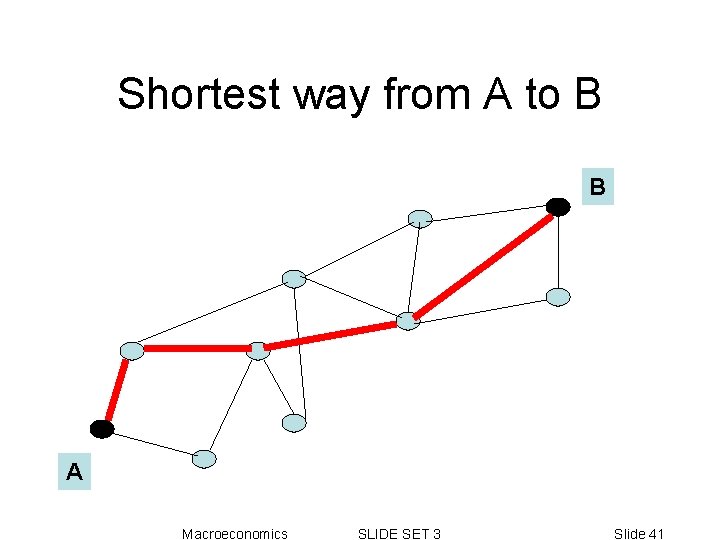
Shortest way from A to B B A Macroeconomics SLIDE SET 3 Slide 41

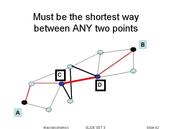
Must be the shortest way between ANY two points B C D A Macroeconomics SLIDE SET 3 Slide 42

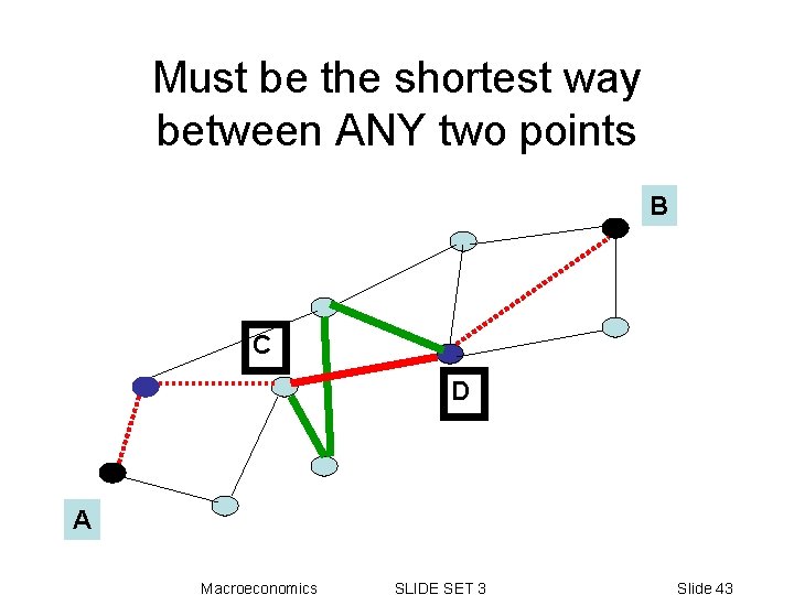
Must be the shortest way between ANY two points B C D A Macroeconomics SLIDE SET 3 Slide 43

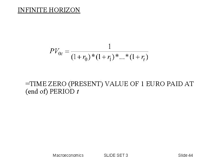
INFINITE HORIZON =TIME ZERO (PRESENT) VALUE OF 1 EURO PAID AT (end of) PERIOD t Macroeconomics SLIDE SET 3 Slide 44

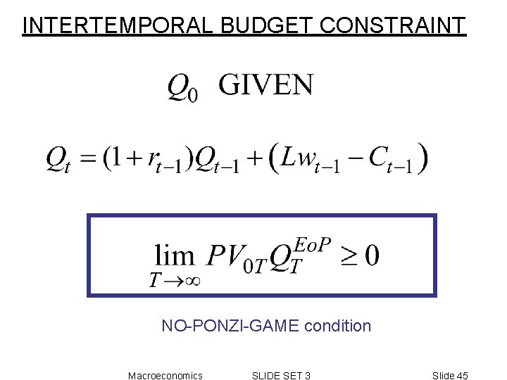
INTERTEMPORAL BUDGET CONSTRAINT NO-PONZI-GAME condition Macroeconomics SLIDE SET 3 Slide 45

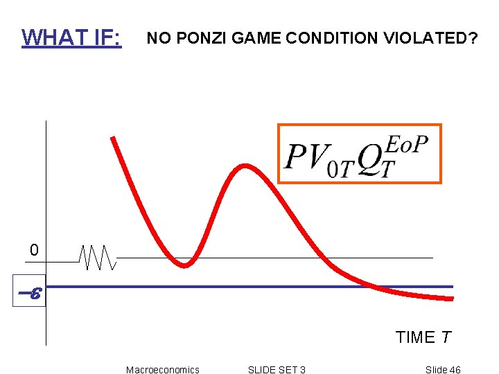
WHAT IF: NO PONZI GAME CONDITION VIOLATED? 0 -e TIME T Macroeconomics SLIDE SET 3 Slide 46

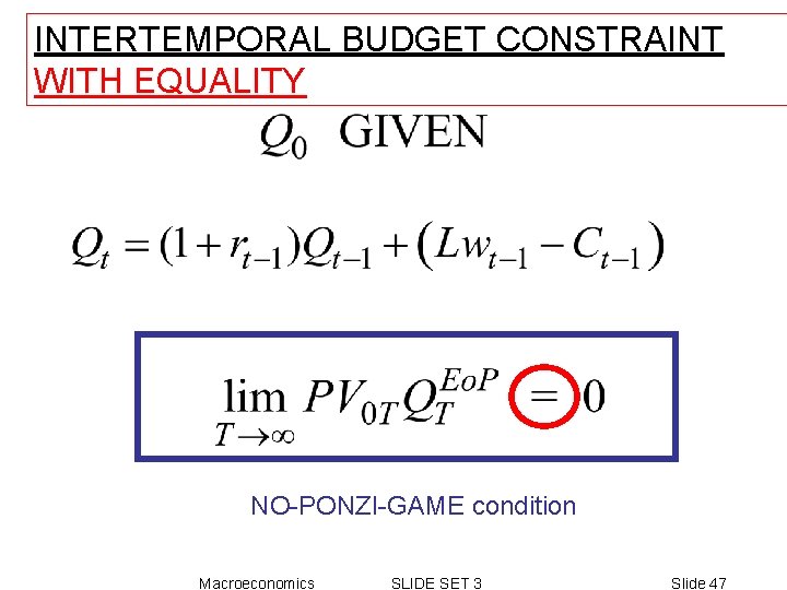
INTERTEMPORAL BUDGET CONSTRAINT WITH EQUALITY NO-PONZI-GAME condition Macroeconomics SLIDE SET 3 Slide 47

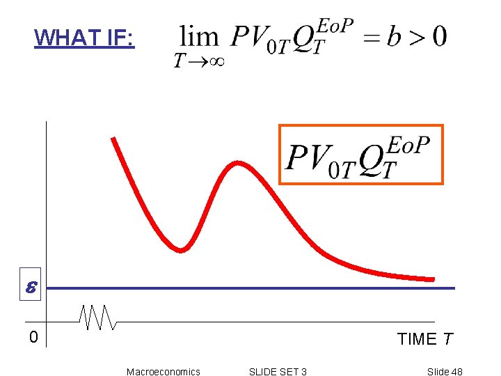
WHAT IF: e 0 TIME T Macroeconomics SLIDE SET 3 Slide 48

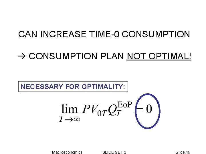
CAN INCREASE TIME-0 CONSUMPTION PLAN NOT OPTIMAL! NECESSARY FOR OPTIMALITY: Macroeconomics SLIDE SET 3 Slide 49

TIME CONSISTENCY of HOUSOLD CONSUMPTION PLANS Macroeconomics SLIDE SET 3 Slide 50

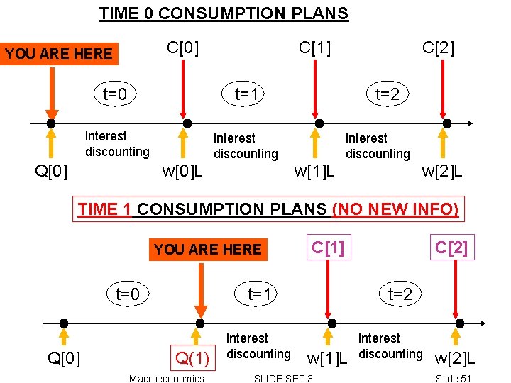
TIME 0 CONSUMPTION PLANS C[0] YOU ARE HERE C[1] t=0 t=1 interest discounting Q[0] w[0]L C[2] t=2 interest discounting w[1]L w[2]L TIME 1 CONSUMPTION PLANS (NO NEW INFO) YOU ARE HERE t=0 Q[0] C[1] t=1 Q(1) Macroeconomics interest discounting C[2] t=2 w[1]L SLIDE SET 3 interest discounting w[2]L Slide 51

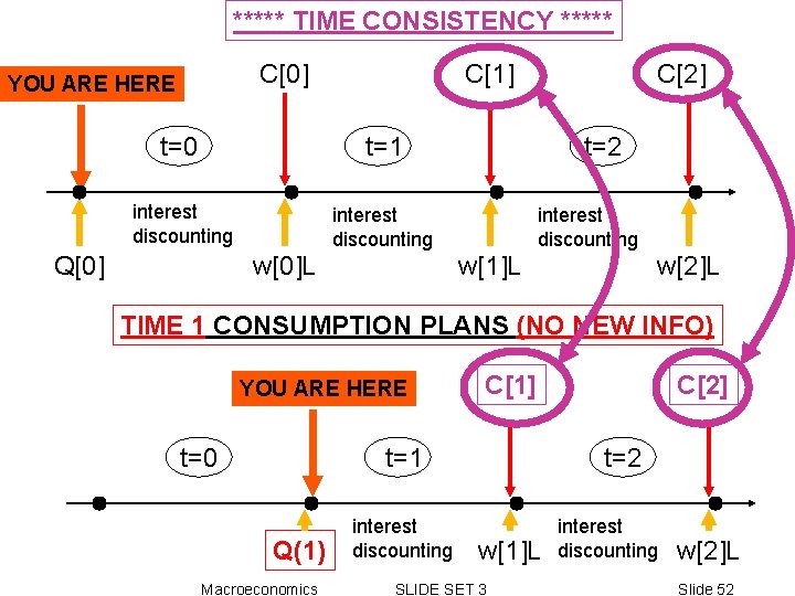
***** TIME CONSISTENCY ***** C[0] YOU ARE HERE C[1] t=0 t=1 interest discounting Q[0] w[0]L C[2] t=2 interest discounting w[1]L w[2]L TIME 1 CONSUMPTION PLANS (NO NEW INFO) YOU ARE HERE t=0 C[1] t=1 Q(1) Macroeconomics interest discounting C[2] t=2 w[1]L SLIDE SET 3 interest discounting w[2]L Slide 52

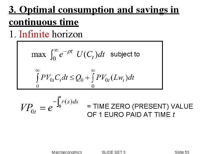
3. Optimal consumption and savings in continuous time 1. Infinite horizon subject to = TIME ZERO (PRESENT) VALUE OF 1 EURO PAID AT TIME t Macroeconomics SLIDE SET 3 Slide 53

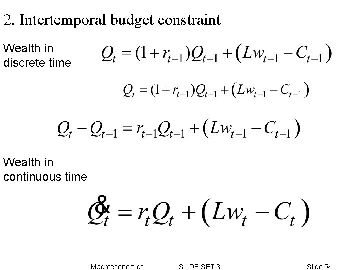
2. Intertemporal budget constraint Wealth in discrete time Wealth in continuous time Macroeconomics SLIDE SET 3 Slide 54

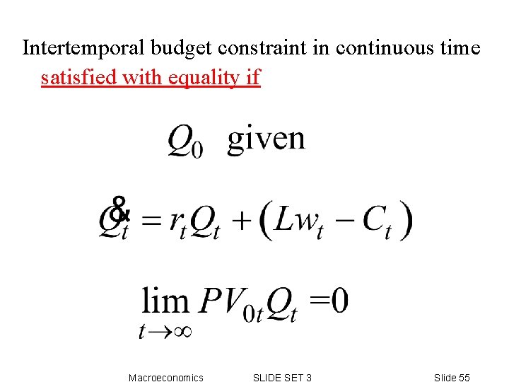
Intertemporal budget constraint in continuous time satisfied with equality if Macroeconomics SLIDE SET 3 Slide 55

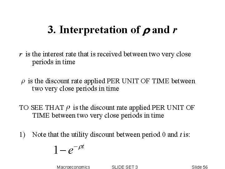
3. Interpretation of r and r r is the interest rate that is received between two very close periods in time is the discount rate applied PER UNIT OF TIME between two very close periods in time TO SEE THAT is the discount rate applied PER UNIT OF TIME between two very close periods in time 1) Note that the utility discount between period 0 and t is: Macroeconomics SLIDE SET 3 Slide 56

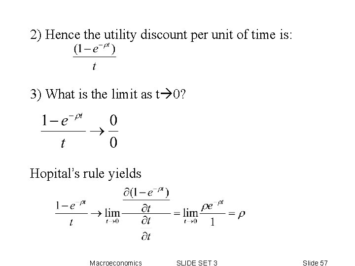
2) Hence the utility discount per unit of time is: 3) What is the limit as t 0? Hopital’s rule yields Macroeconomics SLIDE SET 3 Slide 57

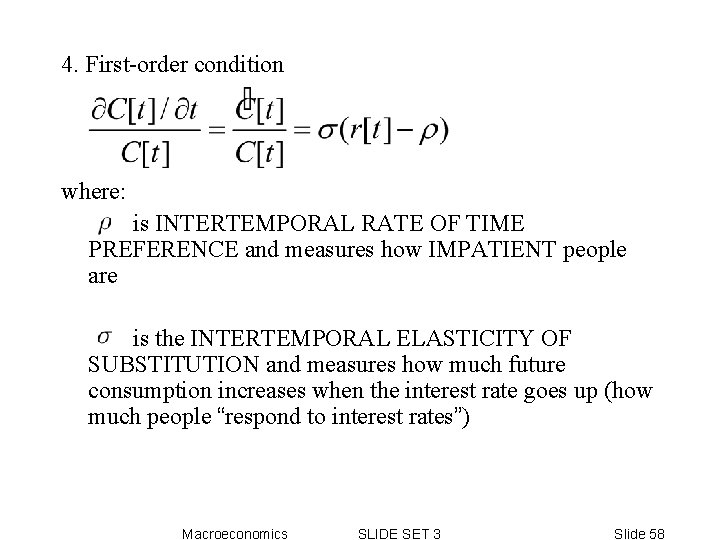
4. First-order condition where: is INTERTEMPORAL RATE OF TIME PREFERENCE and measures how IMPATIENT people are is the INTERTEMPORAL ELASTICITY OF SUBSTITUTION and measures how much future consumption increases when the interest rate goes up (how much people “respond to interest rates”) Macroeconomics SLIDE SET 3 Slide 58

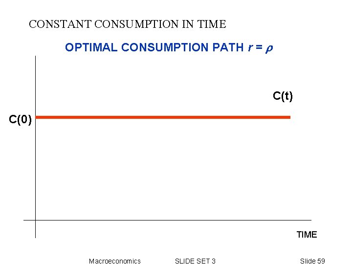
CONSTANT CONSUMPTION IN TIME OPTIMAL CONSUMPTION PATH r = r C(t) C(0) TIME Macroeconomics SLIDE SET 3 Slide 59

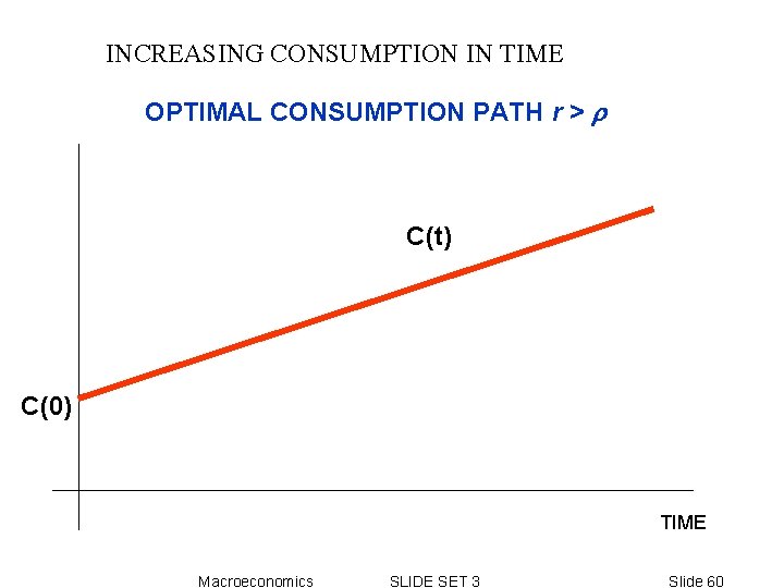
INCREASING CONSUMPTION IN TIME OPTIMAL CONSUMPTION PATH r > r C(t) C(0) TIME Macroeconomics SLIDE SET 3 Slide 60

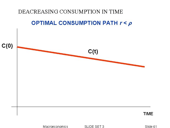
DEACREASING CONSUMPTION IN TIME OPTIMAL CONSUMPTION PATH r < r C(0) C(t) TIME Macroeconomics SLIDE SET 3 Slide 61

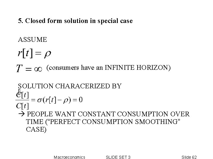
5. Closed form solution in special case ASSUME (consumers have an INFINITE HORIZON) SOLUTION CHARACERIZED BY PEOPLE WANT CONSTANT CONSUMPTION OVER TIME (“PERFECT CONSUMPTION SMOOTHING” CASE) Macroeconomics SLIDE SET 3 Slide 62

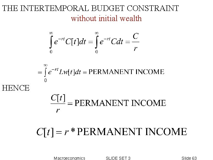
THE INTERTEMPORAL BUDGET CONSTRAINT without initial wealth HENCE Macroeconomics SLIDE SET 3 Slide 63

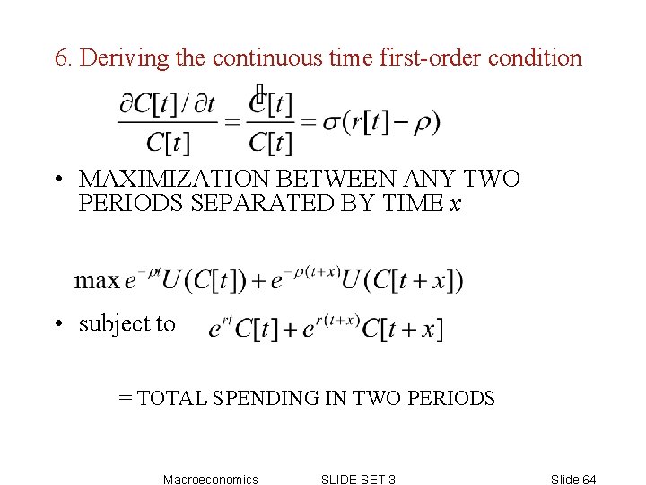
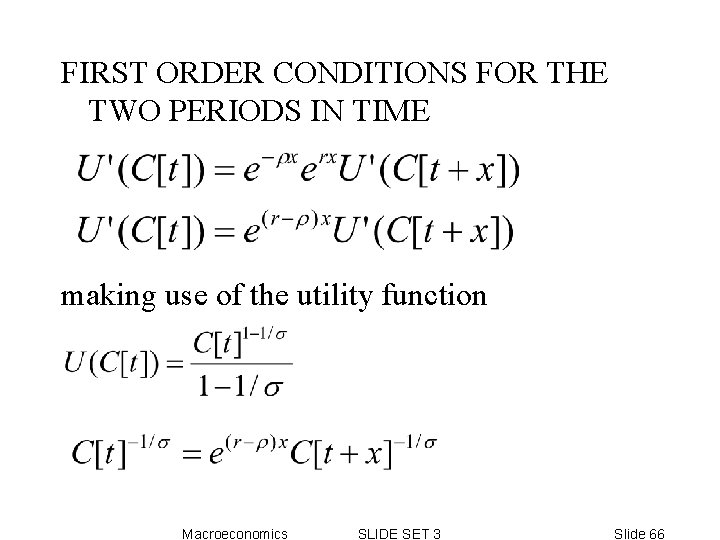
6. Deriving the continuous time first-order condition • MAXIMIZATION BETWEEN ANY TWO PERIODS SEPARATED BY TIME x • subject to = TOTAL SPENDING IN TWO PERIODS Macroeconomics SLIDE SET 3 Slide 64

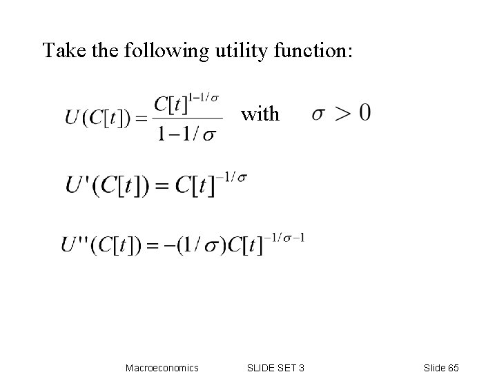
Take the following utility function: with Macroeconomics SLIDE SET 3 Slide 65

FIRST ORDER CONDITIONS FOR THE TWO PERIODS IN TIME making use of the utility function Macroeconomics SLIDE SET 3 Slide 66

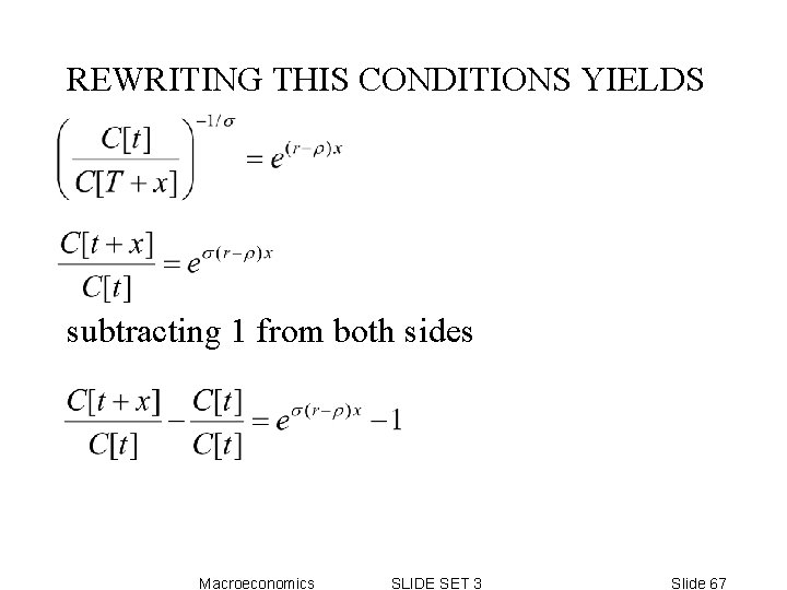
REWRITING THIS CONDITIONS YIELDS subtracting 1 from both sides Macroeconomics SLIDE SET 3 Slide 67

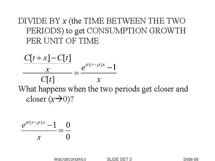
DIVIDE BY x (the TIME BETWEEN THE TWO PERIODS) to get CONSUMPTION GROWTH PER UNIT OF TIME What happens when the two periods get closer and closer (x 0)? Macroeconomics SLIDE SET 3 Slide 68

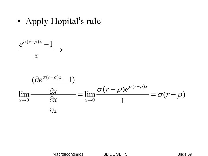
• Apply Hopital’s rule Macroeconomics SLIDE SET 3 Slide 69

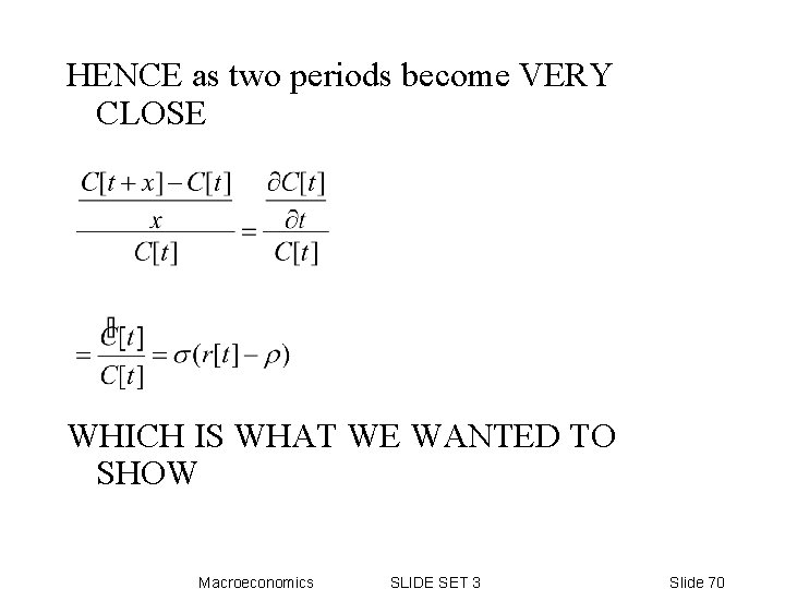
HENCE as two periods become VERY CLOSE WHICH IS WHAT WE WANTED TO SHOW Macroeconomics SLIDE SET 3 Slide 70

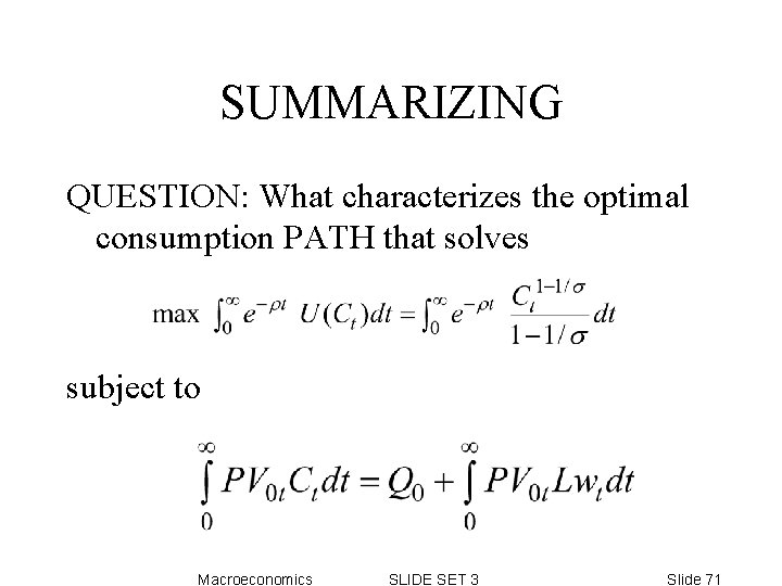
SUMMARIZING QUESTION: What characterizes the optimal consumption PATH that solves subject to Macroeconomics SLIDE SET 3 Slide 71

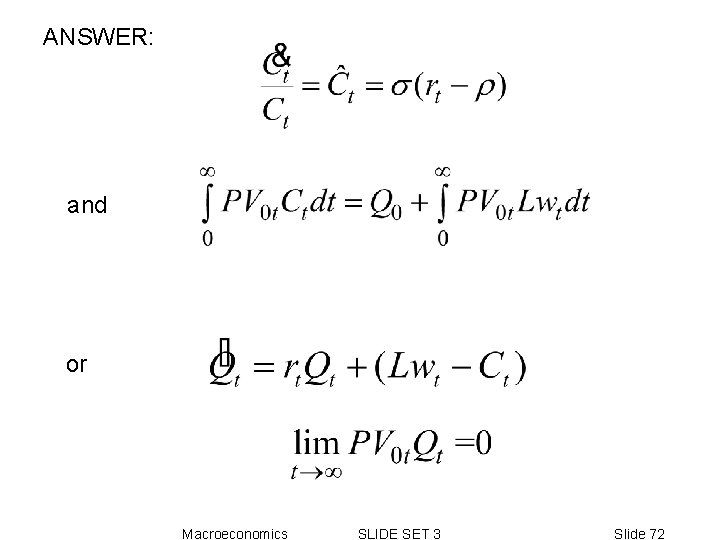
ANSWER: and or Macroeconomics SLIDE SET 3 Slide 72

2. The Ramsey-Cass-Koopmans model Macroeconomics SLIDE SET 3 Slide 73

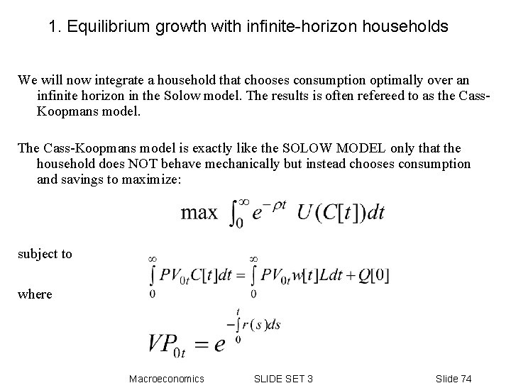
1. Equilibrium growth with infinite-horizon households We will now integrate a household that chooses consumption optimally over an infinite horizon in the Solow model. The results is often refereed to as the Cass. Koopmans model. The Cass-Koopmans model is exactly like the SOLOW MODEL only that the household does NOT behave mechanically but instead chooses consumption and savings to maximize: subject to where Macroeconomics SLIDE SET 3 Slide 74

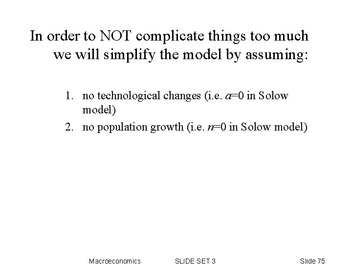
In order to NOT complicate things too much we will simplify the model by assuming: 1. no technological changes (i. e. a=0 in Solow model) 2. no population growth (i. e. n=0 in Solow model) Macroeconomics SLIDE SET 3 Slide 75

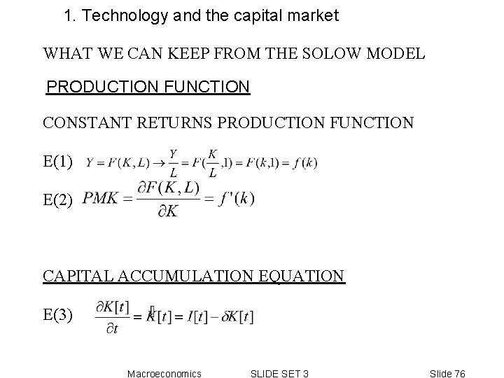
1. Technology and the capital market WHAT WE CAN KEEP FROM THE SOLOW MODEL PRODUCTION FUNCTION CONSTANT RETURNS PRODUCTION FUNCTION E(1) E(2) CAPITAL ACCUMULATION EQUATION E(3) Macroeconomics SLIDE SET 3 Slide 76

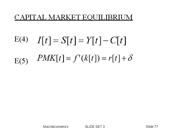
CAPITAL MARKET EQUILIBRIUM E(4) E(5) Macroeconomics SLIDE SET 3 Slide 77

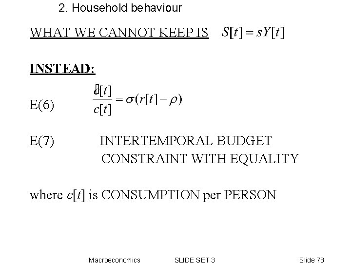
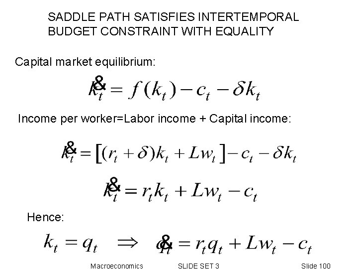
2. Household behaviour WHAT WE CANNOT KEEP IS INSTEAD: E(6) E(7) INTERTEMPORAL BUDGET CONSTRAINT WITH EQUALITY where c[t] is CONSUMPTION per PERSON Macroeconomics SLIDE SET 3 Slide 78

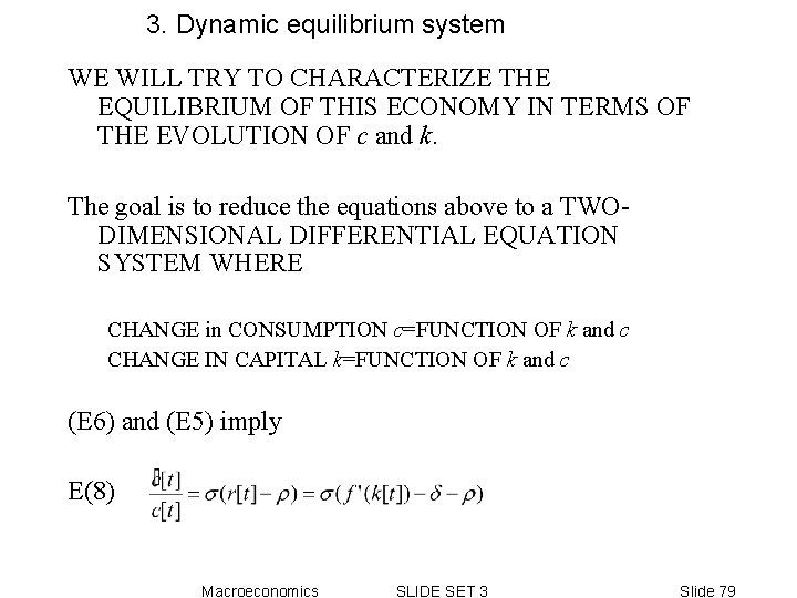
3. Dynamic equilibrium system WE WILL TRY TO CHARACTERIZE THE EQUILIBRIUM OF THIS ECONOMY IN TERMS OF THE EVOLUTION OF c and k. The goal is to reduce the equations above to a TWODIMENSIONAL DIFFERENTIAL EQUATION SYSTEM WHERE CHANGE in CONSUMPTION c=FUNCTION OF k and c CHANGE IN CAPITAL k=FUNCTION OF k and c (E 6) and (E 5) imply E(8) Macroeconomics SLIDE SET 3 Slide 79

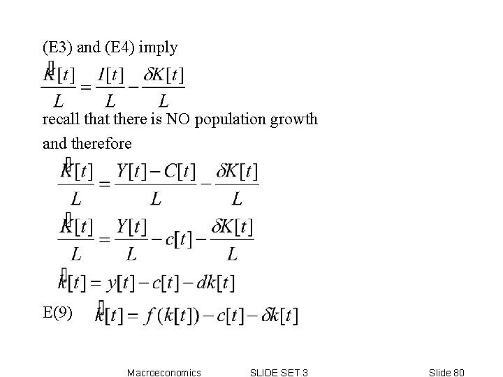
(E 3) and (E 4) imply recall that there is NO population growth and therefore E(9) Macroeconomics SLIDE SET 3 Slide 80

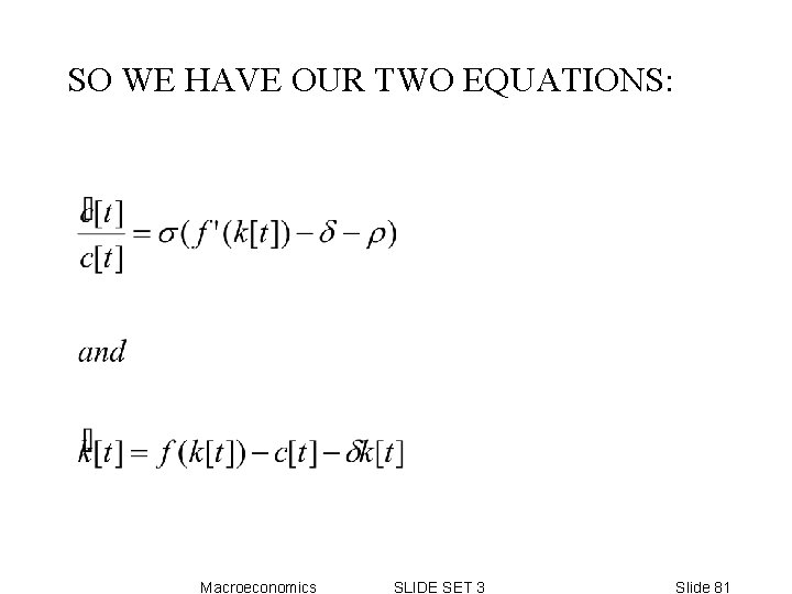
SO WE HAVE OUR TWO EQUATIONS: Macroeconomics SLIDE SET 3 Slide 81

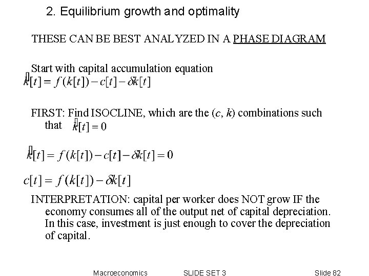
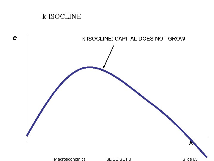
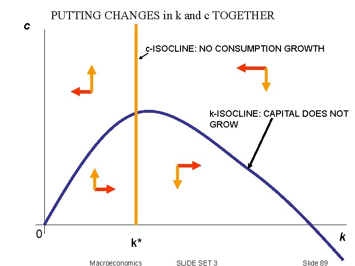
2. Equilibrium growth and optimality THESE CAN BE BEST ANALYZED IN A PHASE DIAGRAM Start with capital accumulation equation FIRST: Find ISOCLINE, which are the (c, k) combinations such that INTERPRETATION: capital per worker does NOT grow IF the economy consumes all of the output net of capital depreciation. In this case, investment is just enough to cover the depreciation of capital. Macroeconomics SLIDE SET 3 Slide 82

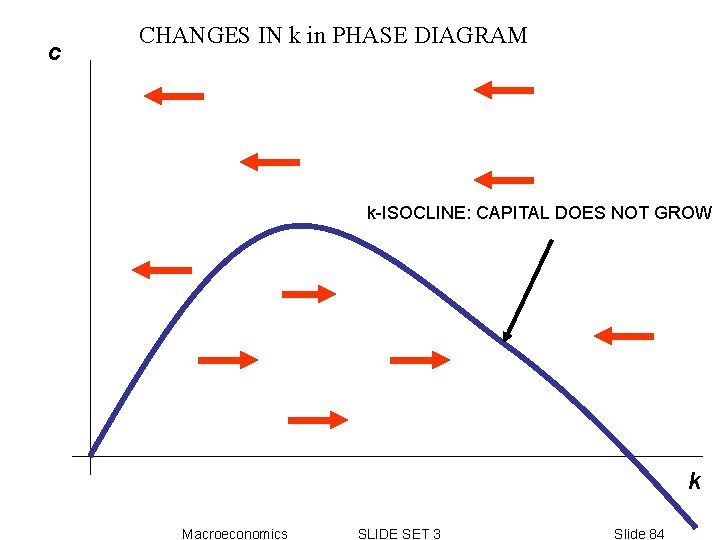
k-ISOCLINE c k-ISOCLINE: CAPITAL DOES NOT GROW k Macroeconomics SLIDE SET 3 Slide 83

c CHANGES IN k in PHASE DIAGRAM k-ISOCLINE: CAPITAL DOES NOT GROW k Macroeconomics SLIDE SET 3 Slide 84

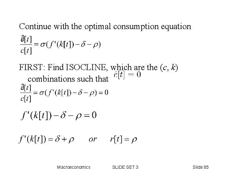
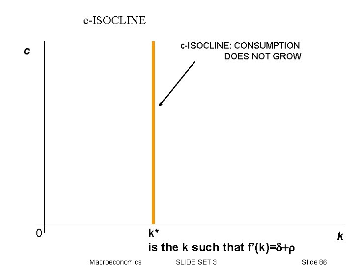
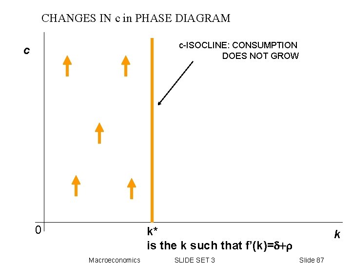
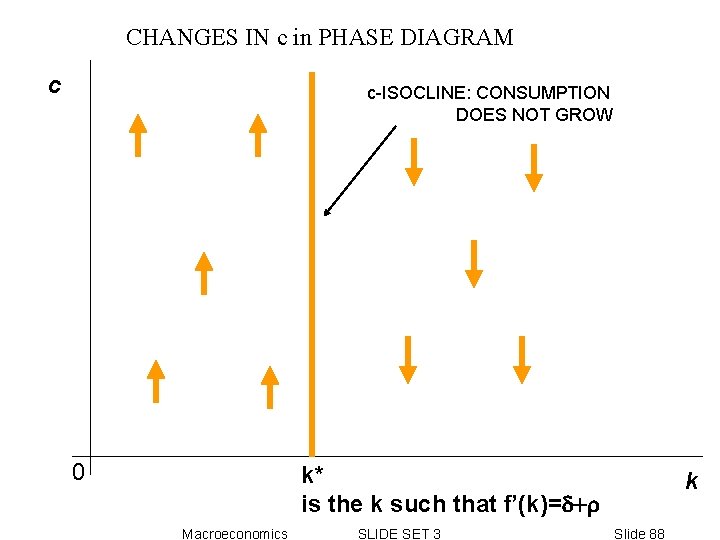
Continue with the optimal consumption equation FIRST: Find ISOCLINE, which are the (c, k) combinations such that Macroeconomics SLIDE SET 3 Slide 85

c-ISOCLINE: CONSUMPTION DOES NOT GROW c 0 k* is the k such that f’(k)=d+r Macroeconomics SLIDE SET 3 k Slide 86

CHANGES IN c in PHASE DIAGRAM c-ISOCLINE: CONSUMPTION DOES NOT GROW c 0 k* is the k such that f’(k)=d+r Macroeconomics SLIDE SET 3 k Slide 87

CHANGES IN c in PHASE DIAGRAM c c-ISOCLINE: CONSUMPTION DOES NOT GROW 0 k* is the k such that f’(k)=d+r Macroeconomics SLIDE SET 3 k Slide 88

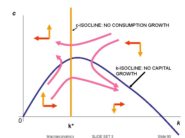
PUTTING CHANGES in k and c TOGETHER c c-ISOCLINE: NO CONSUMPTION GROWTH k-ISOCLINE: CAPITAL DOES NOT GROW 0 k k* Macroeconomics SLIDE SET 3 Slide 89

c c-ISOCLINE: NO CONSUMPTION GROWTH k-ISOCLINE: NO CAPITAL GROWTH 0 k k* Macroeconomics SLIDE SET 3 Slide 90

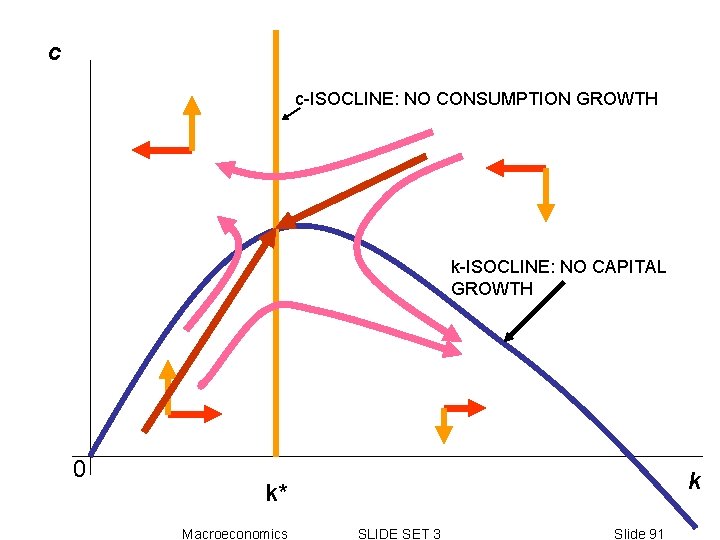
c c-ISOCLINE: NO CONSUMPTION GROWTH k-ISOCLINE: NO CAPITAL GROWTH 0 k k* Macroeconomics SLIDE SET 3 Slide 91

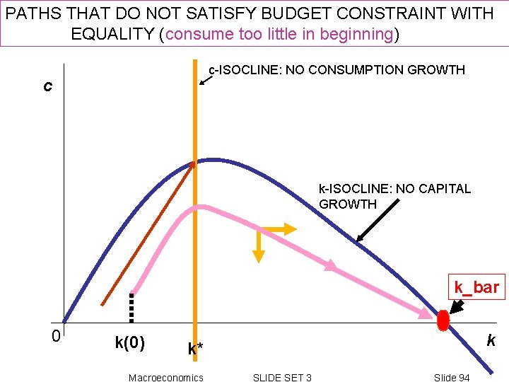
All these paths satisfy by construction: -period-by-period consumer maximization -capital market equilibrium They DO NOT necessarily satisfy constraints like: -non-negative capital stock k[t]>=0 -intertemporal budget constraint with EQUALITY Macroeconomics SLIDE SET 3 Slide 92

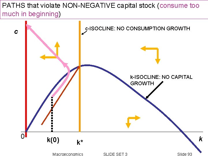
PATHS that violate NON-NEGATIVE capital stock (consume too much in beginning) c-ISOCLINE: NO CONSUMPTION GROWTH c k-ISOCLINE: NO CAPITAL GROWTH 0 k(0) k k* Macroeconomics SLIDE SET 3 Slide 93

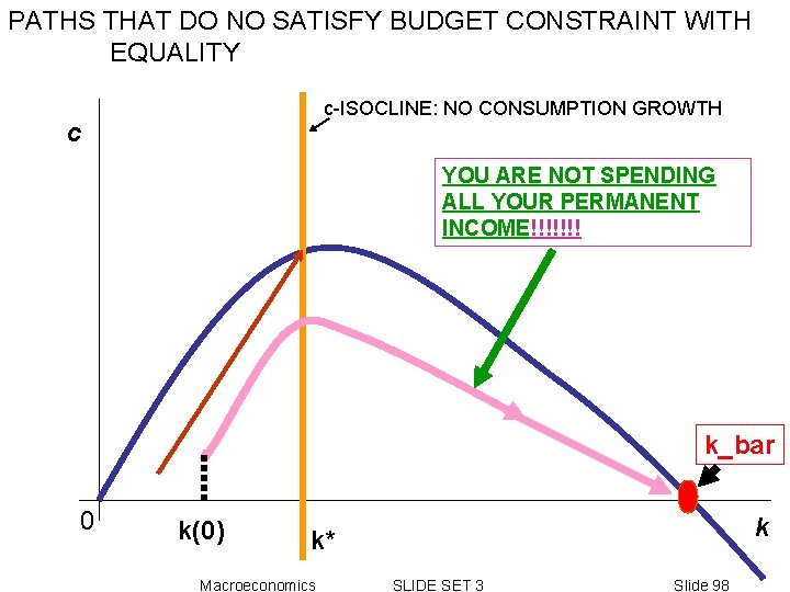
PATHS THAT DO NOT SATISFY BUDGET CONSTRAINT WITH EQUALITY (consume too little in beginning) c-ISOCLINE: NO CONSUMPTION GROWTH c k-ISOCLINE: NO CAPITAL GROWTH k_bar 0 k(0) k k* Macroeconomics SLIDE SET 3 Slide 94

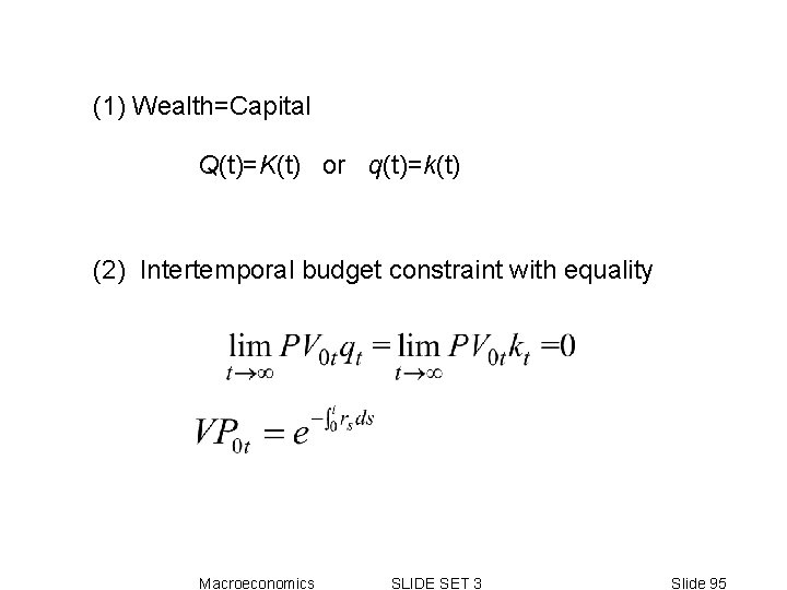
(1) Wealth=Capital Q(t)=K(t) or q(t)=k(t) (2) Intertemporal budget constraint with equality Macroeconomics SLIDE SET 3 Slide 95

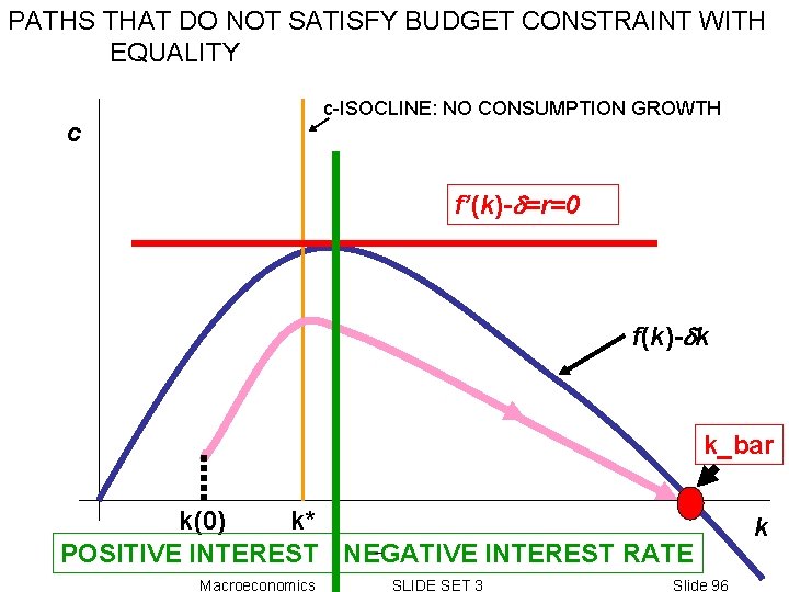
PATHS THAT DO NOT SATISFY BUDGET CONSTRAINT WITH EQUALITY c-ISOCLINE: NO CONSUMPTION GROWTH c f’(k)-d=r=0 f(k)-dk k_bar k(0) k* POSITIVE INTEREST NEGATIVE INTEREST RATE Macroeconomics SLIDE SET 3 Slide 96 k

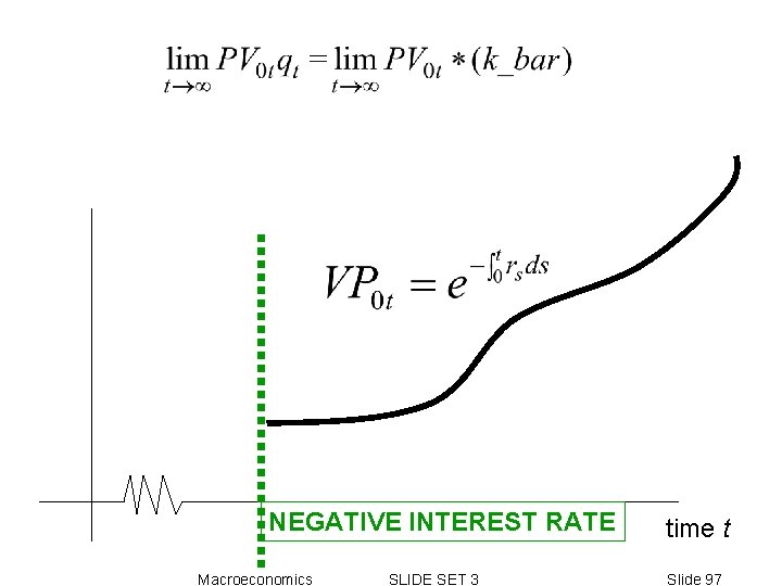
NEGATIVE INTEREST RATE Macroeconomics SLIDE SET 3 time t Slide 97

PATHS THAT DO NO SATISFY BUDGET CONSTRAINT WITH EQUALITY c-ISOCLINE: NO CONSUMPTION GROWTH c YOU ARE NOT SPENDING ALL YOUR PERMANENT INCOME!!!!!!! k_bar 0 k(0) k k* Macroeconomics SLIDE SET 3 Slide 98

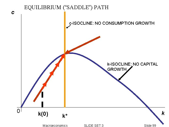
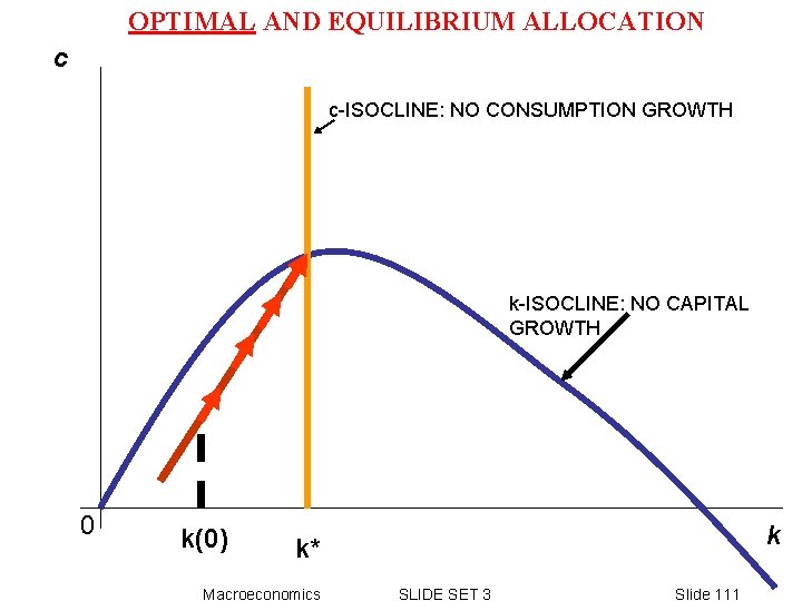
EQUILIBRIUM (“SADDLE”) PATH c c-ISOCLINE: NO CONSUMPTION GROWTH k-ISOCLINE: NO CAPITAL GROWTH 0 k(0) k k* Macroeconomics SLIDE SET 3 Slide 99

SADDLE PATH SATISFIES INTERTEMPORAL BUDGET CONSTRAINT WITH EQUALITY Capital market equilibrium: Income per worker=Labor income + Capital income: Hence: Macroeconomics SLIDE SET 3 Slide 100

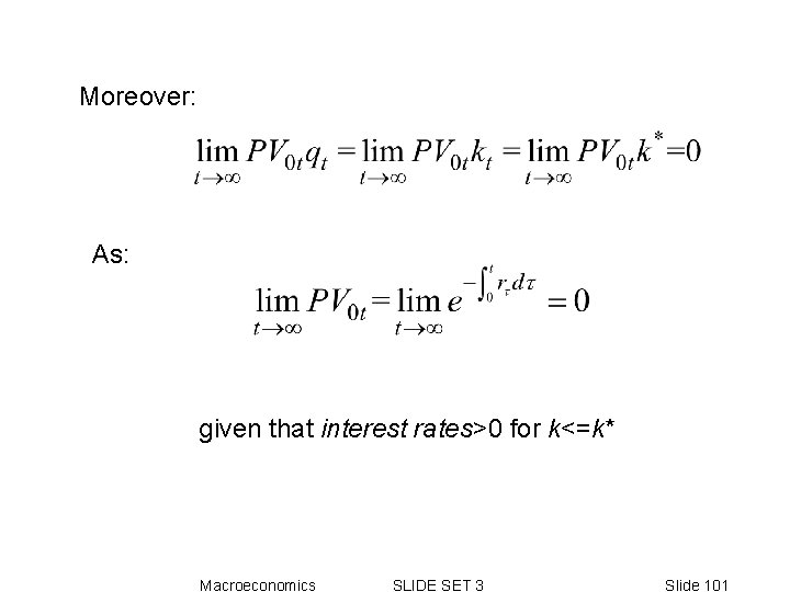
Moreover: As: given that interest rates>0 for k<=k* Macroeconomics SLIDE SET 3 Slide 101

OPTIMALITY -- What would social planner do? - Social planner: dictator who decides allocation according to HH welfare subject to physical contraints Macroeconomics SLIDE SET 3 Slide 102

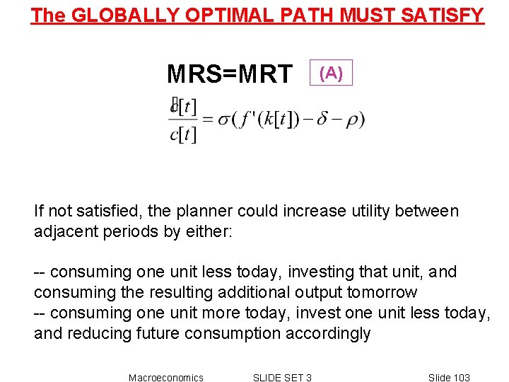
The GLOBALLY OPTIMAL PATH MUST SATISFY MRS=MRT (A) If not satisfied, the planner could increase utility between adjacent periods by either: -- consuming one unit less today, investing that unit, and consuming the resulting additional output tomorrow -- consuming one unit more today, invest one unit less today, and reducing future consumption accordingly Macroeconomics SLIDE SET 3 Slide 103

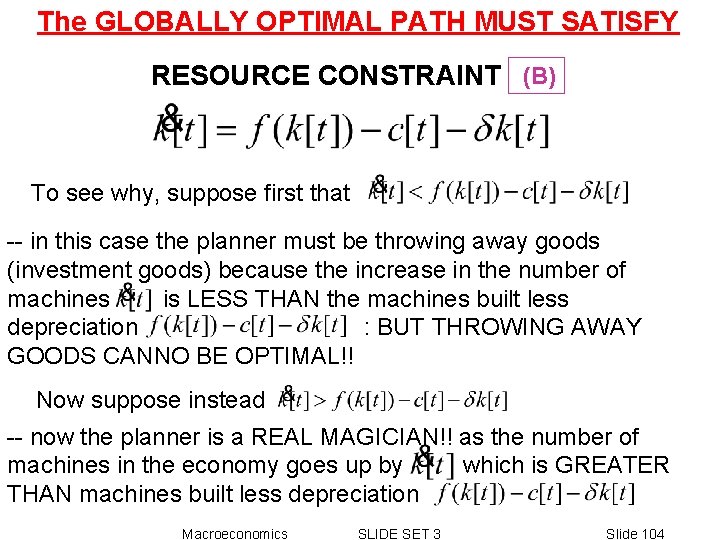
The GLOBALLY OPTIMAL PATH MUST SATISFY RESOURCE CONSTRAINT (B) To see why, suppose first that -- in this case the planner must be throwing away goods (investment goods) because the increase in the number of machines is LESS THAN the machines built less depreciation : BUT THROWING AWAY GOODS CANNO BE OPTIMAL!! Now suppose instead -- now the planner is a REAL MAGICIAN!! as the number of machines in the economy goes up by which is GREATER THAN machines built less depreciation Macroeconomics SLIDE SET 3 Slide 104

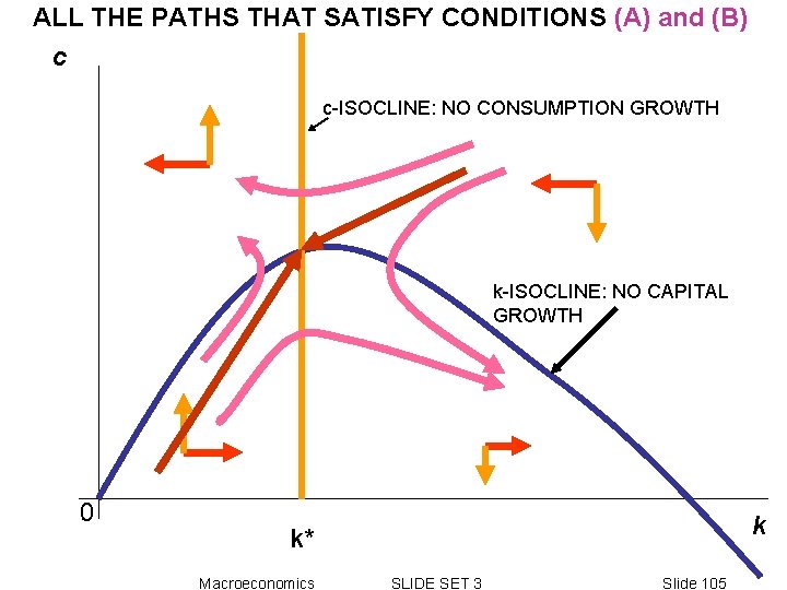
ALL THE PATHS THAT SATISFY CONDITIONS (A) and (B) c c-ISOCLINE: NO CONSUMPTION GROWTH k-ISOCLINE: NO CAPITAL GROWTH 0 k k* Macroeconomics SLIDE SET 3 Slide 105

NOW NOTE: -- Starting the allocation by jumping ABOVE the SADDLE PATH CANNOT BE OPTIMAL because you end up violating the non-negativity constraint for capital -- Starting the allocation by jumping BELOW the SADDLE PATH CANNOT BE OPTIMAL either. The proof is to construct another path—that is clearly not optimal either— but that still is BETTER THAN the paths starting out below the saddle path. How to do that is explained on the next slides. Macroeconomics SLIDE SET 3 Slide 106

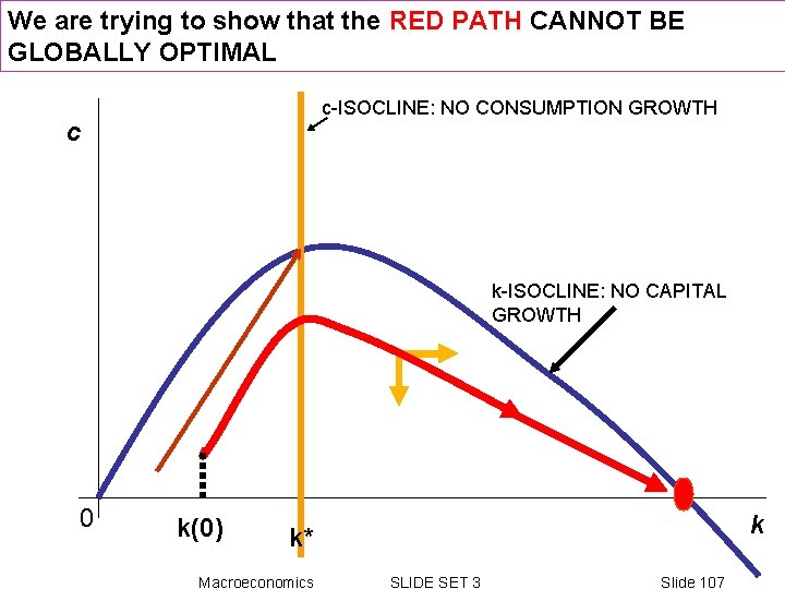
We are trying to show that the RED PATH CANNOT BE GLOBALLY OPTIMAL c-ISOCLINE: NO CONSUMPTION GROWTH c k-ISOCLINE: NO CAPITAL GROWTH 0 k(0) k k* Macroeconomics SLIDE SET 3 Slide 107

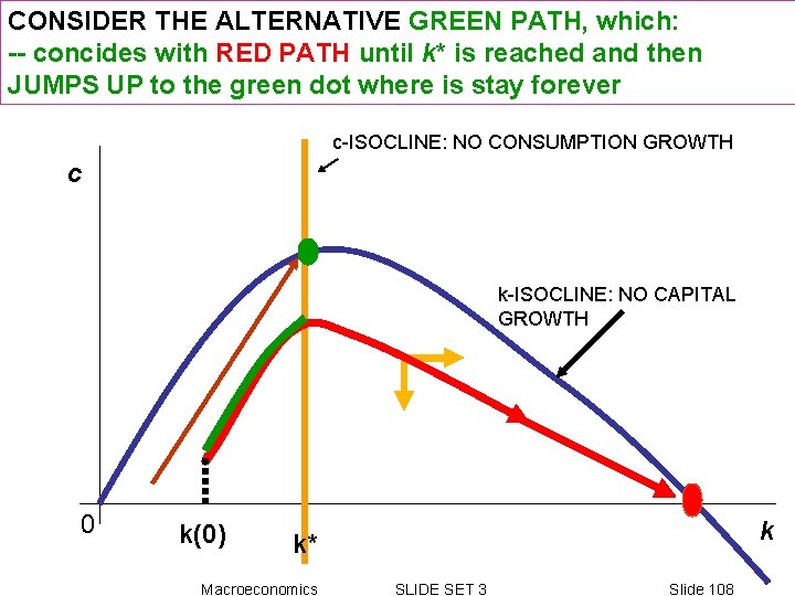
CONSIDER THE ALTERNATIVE GREEN PATH, which: -- concides with RED PATH until k* is reached and then JUMPS UP to the green dot where is stay forever c-ISOCLINE: NO CONSUMPTION GROWTH c k-ISOCLINE: NO CAPITAL GROWTH 0 k(0) k k* Macroeconomics SLIDE SET 3 Slide 108

-- The GREEN PATH CANNOT POSSIBLY BE OPTIMAL because consumption JUMPS and therefore the green path violates CONSUMPTION SMOOTHING, which was CONDITION A above. -- Still, the GREEN PATH is certaintly better than the RED PATH because it has the same consumption until k* and MORE consumption from there onwards!!! -- For all RED PATHS (that is, all paths starting below the saddle path), there is a GREEN PATH. So no paths starting below the saddle path can be optimal (despite the fact that it satisfies conditions A and B). Macroeconomics SLIDE SET 3 Slide 109

HENCE: The only path starting at k[0] that : -- satisfies CONDITIONS A and B, which are necessary for optimality -- satisfies non-negativity of capital -- satisfies that there is NO OTHER PATH we can construct that is better IS THE SADDLE PATH EQUILIBRIUM AND OPTIMAL ALLOCATIONS ARE EQUAL Macroeconomics SLIDE SET 3 Slide 110

OPTIMAL AND EQUILIBRIUM ALLOCATION c c-ISOCLINE: NO CONSUMPTION GROWTH k-ISOCLINE: NO CAPITAL GROWTH 0 k(0) k k* Macroeconomics SLIDE SET 3 Slide 111

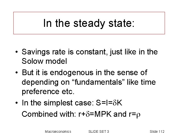
In the steady state: • Savings rate is constant, just like in the Solow model • But it is endogenous in the sense of depending on “fundamentals” like time preference etc. • In the simplest case: S=I=d. K Combined with: r+d=MPK and r=r Macroeconomics SLIDE SET 3 Slide 112

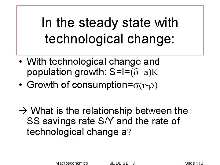
In the steady state with technological change: • With technological change and population growth: S=I=(d+a)K • Growth of consumption=s(r-r) What is the relationship between the SS savings rate S/Y and the rate of technological change a? Macroeconomics SLIDE SET 3 Slide 113

Comparative statics • Greater impatience (discount rate)? (effects on income, capital, wages, interest rates) • Capital income taxation? • A temporary cut of lump-sum taxes? Macroeconomics SLIDE SET 3 Slide 114