AP Macroeconomics Graphs in order to survive Mr

AP Macroeconomics Graphs in order to survive Mr. Forrest’s class By: Martin Malimban Class of 2013

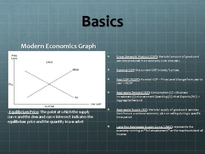
Basics Modern Economics Graph Gross Domestic Product (GDP): the total amount of goods and services produced in an economy over one year. Nominal GDP: the current GDP in today’s prices Real GDP (RGDP): Nominal GDP – Price Level Change from year to year = RGDP Aggregate Demand (AD): Consumption (C) + Business Investment (I) +Government Spending (G) +Net Exports (NX) = Aggregate Demand - Equilibrium Price: The point at which the supply curve and the demand curve intersect indicates the equilibrium price and the quantity in a market Aggregate Supply (AS): the total supply of goods and services that firms in a national economy plan on selling during a specific time period Long Run Aggregate Supply Curve (LRAS): represents the economy running at “full employment” or the maximum level of income

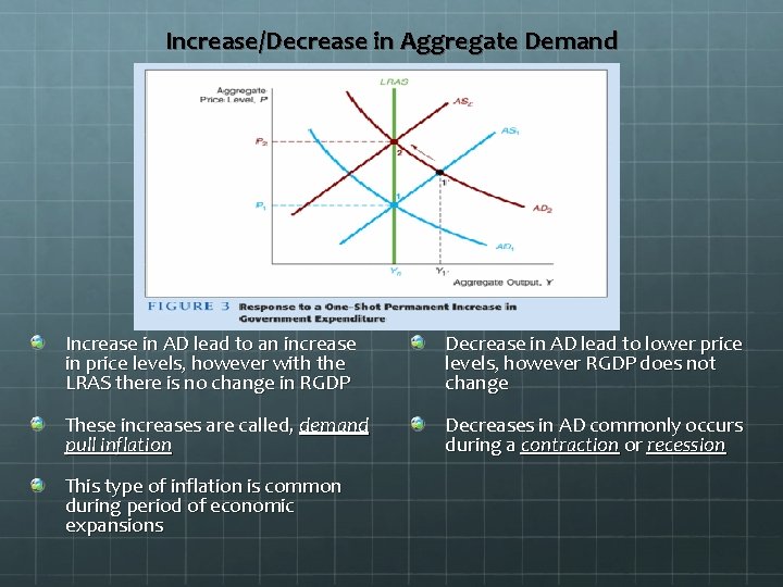
Increase/Decrease in Aggregate Demand Increase in AD lead to an increase in price levels, however with the LRAS there is no change in RGDP Decrease in AD lead to lower price levels, however RGDP does not change These increases are called, demand pull inflation Decreases in AD commonly occurs during a contraction or recession This type of inflation is common during period of economic expansions

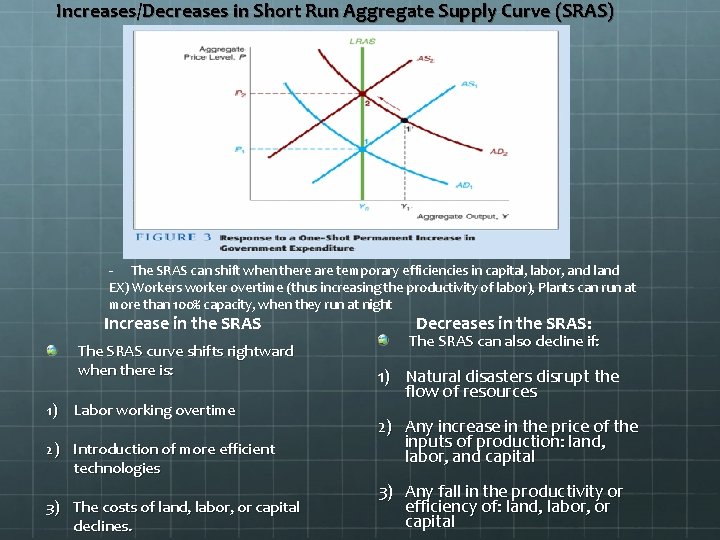
Increases/Decreases in Short Run Aggregate Supply Curve (SRAS) - The SRAS can shift when there are temporary efficiencies in capital, labor, and land EX) Workers worker overtime (thus increasing the productivity of labor), Plants can run at more than 100% capacity, when they run at night Increase in the SRAS The SRAS curve shifts rightward when there is: 1) Labor working overtime 2) Introduction of more efficient technologies 3) The costs of land, labor, or capital declines. Decreases in the SRAS: The SRAS can also decline if: 1) Natural disasters disrupt the flow of resources 2) Any increase in the price of the inputs of production: land, labor, and capital 3) Any fall in the productivity or efficiency of: land, labor, or capital

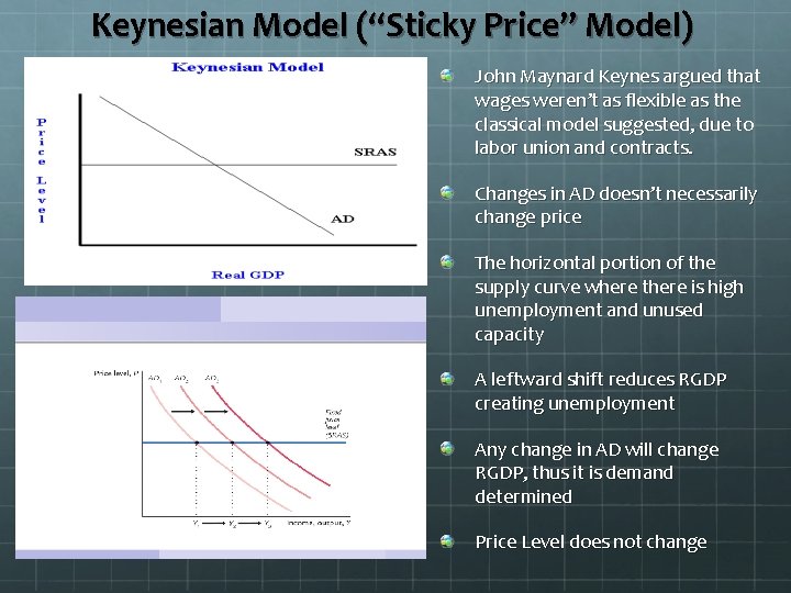
Keynesian Model (“Sticky Price” Model) John Maynard Keynes argued that wages weren’t as flexible as the classical model suggested, due to labor union and contracts. Changes in AD doesn’t necessarily change price The horizontal portion of the supply curve where there is high unemployment and unused capacity A leftward shift reduces RGDP creating unemployment Any change in AD will change RGDP, thus it is demand determined Price Level does not change

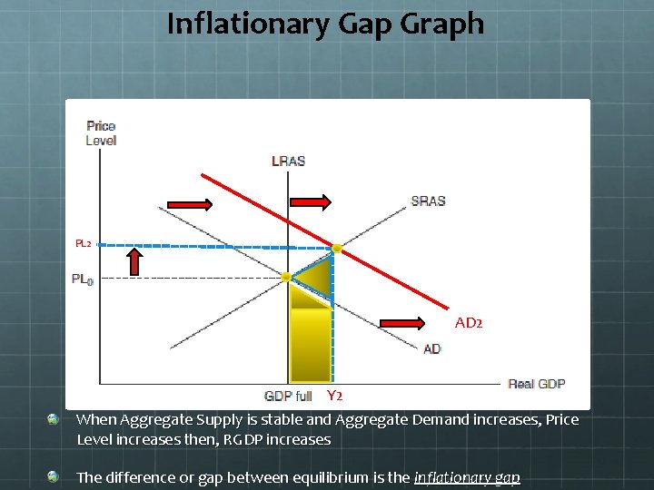
Inflationary Gap Graph PL 22 AD 2 Y 2 When Aggregate Supply is stable and Aggregate Demand increases, Price Level increases then, RGDP increases The difference or gap between equilibrium is the inflationary gap

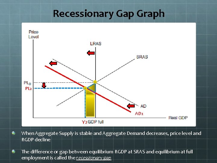
Recessionary Gap Graph PL 2 AD 2 Y 2 When Aggregate Supply is stable and Aggregate Demand decreases, price level and RGDP decline The difference or gap between equilibrium RGDP at SRAS and equilibrium at full employment is called the recessionary gap

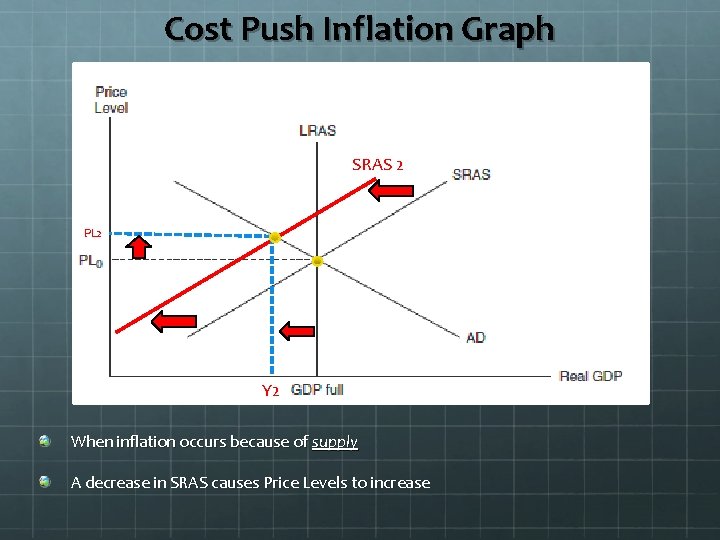
Cost Push Inflation Graph SRAS 2 PL 2 Y 2 When inflation occurs because of supply A decrease in SRAS causes Price Levels to increase

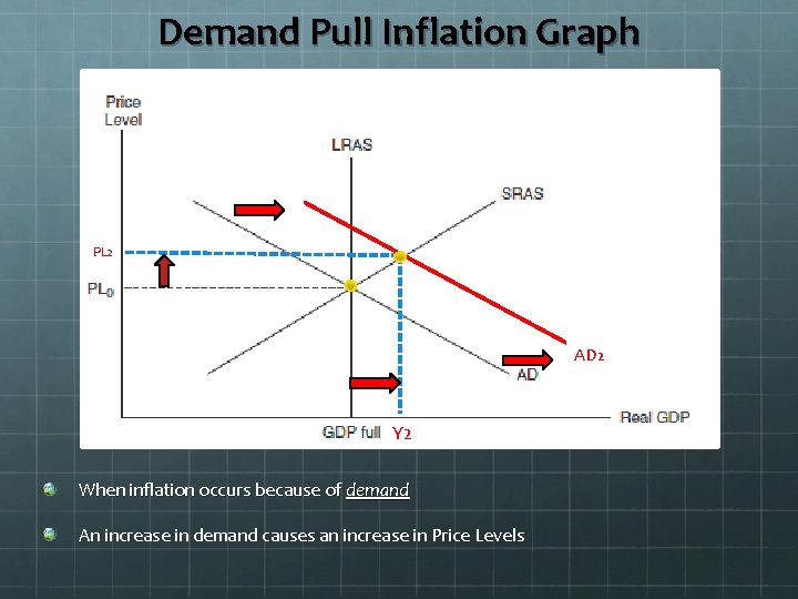
Demand Pull Inflation Graph PL 2 AD 2 Y 2 When inflation occurs because of demand An increase in demand causes an increase in Price Levels

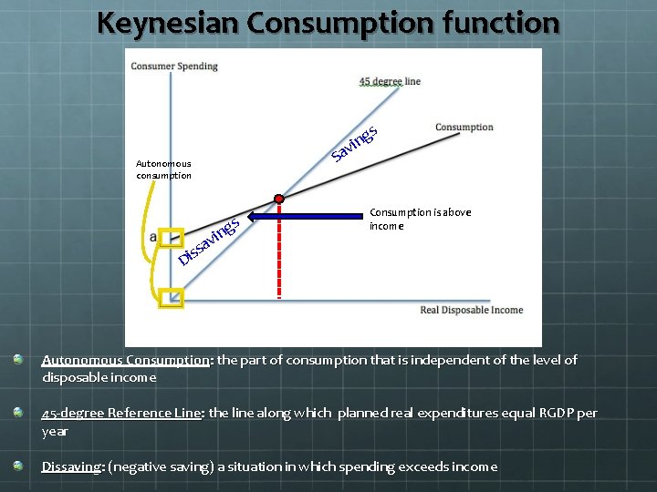
Keynesian Consumption function s g n i v Sa Autonomous consumption Di s g n vi a s s Consumption is above income Autonomous Consumption: the part of consumption that is independent of the level of disposable income 45 -degree Reference Line: the line along which planned real expenditures equal RGDP per year Dissaving: (negative saving) a situation in which spending exceeds income

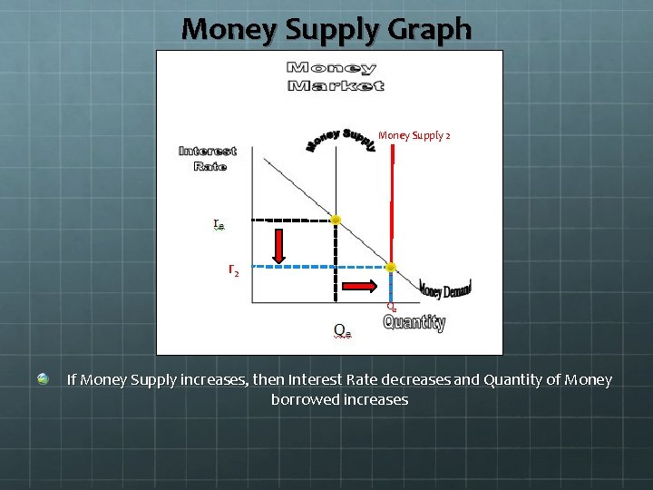
Money Supply Graph Money Supply 2 r 2 Q 2 If Money Supply increases, then Interest Rate decreases and Quantity of Money borrowed increases

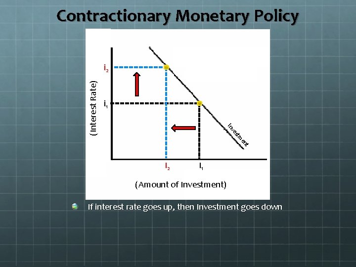
Contractionary Monetary Policy i 1 en tm es v In (Interest Rate) i 2 t I 2 I 1 (Amount of Investment) If interest rate goes up, then Investment goes down

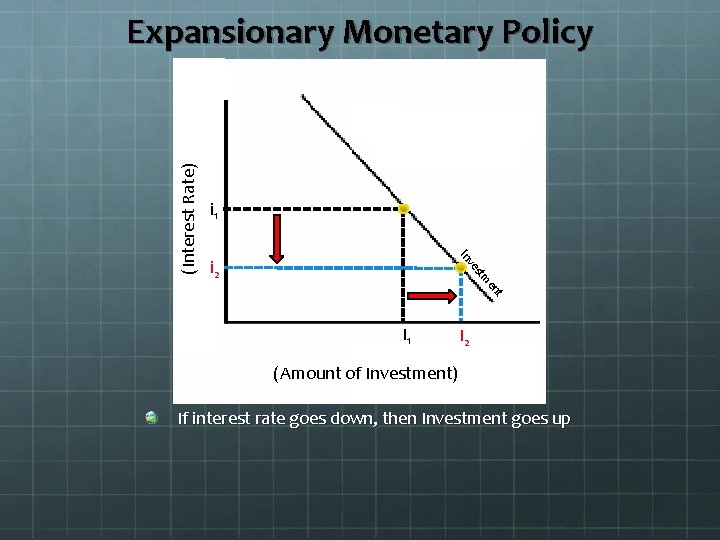
i 1 v In i 2 en tm es (Interest Rate) Expansionary Monetary Policy t I 1 I 2 (Amount of Investment) If interest rate goes down, then Investment goes up

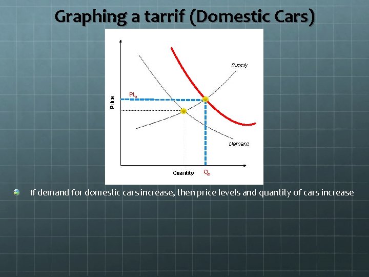
Graphing a tarrif (Domestic Cars) PL 2 Q 2 If demand for domestic cars increase, then price levels and quantity of cars increase

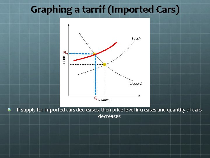
Graphing a tarrif (Imported Cars) PL 2 Q 2 If supply for imported cars decreases, then price level increases and quantity of cars decreases