Mc Eachern Macroeconomics 11 e Ch 10 10

Mc. Eachern, Macroeconomics 11 e, Ch. 10 10 Aggregate Supply Prepared by: V. Andreea Chiritescu, Eastern Illinois University Reviewed by: William A. Mc. Eachern, University of Connecticut © 2017 Cengage Learning®. May not be scanned, copied or duplicated, or posted to a publicly accessible website, in whole or in part.

Mc. Eachern, Macroeconomics 11 e, Ch. 10 • How do producers react when the economy's price level increases? • If the economy is already operating at full employment, how can it produce more? • What's your normal capacity for academic work, and when do you exceed that effort? • What valuable piece of information do employers and workers lack when they negotiate wages? • Why do employers and workers fail to agree on pay cuts that could save jobs? © 2017 Cengage Learning®. May not be scanned, copied or duplicated, or posted to a publicly accessible website, in whole or in part.

Aggregate Supply in the Short Run • Aggregate supply, AS – Relationship between the price level – And output firms are willing and able to supply – Other things constant • Resource prices • State of technology and know-how • Rules of the game © 2017 Cengage Learning®. May not be scanned, copied or duplicated, or posted to a publicly accessible website, in whole or in part. Mc. Eachern, Macroeconomics 11 e, Ch. 10

Labor and Aggregate Supply • Labor – Most important resource – Account for about 70% of production costs • Supply of labor depends on – Size and abilities of adult population – Preferences for work versus leisure • Higher wage – More labor supplied © 2017 Cengage Learning®. May not be scanned, copied or duplicated, or posted to a publicly accessible website, in whole or in part. Mc. Eachern, Macroeconomics 11 e, Ch. 10

Labor and Aggregate Supply • Higher price level – The less the money wage purchases – The less attractive that wage to workers • Nominal wage – In dollars of the current year • Real wage – In dollars of constant purchasing power • Wage negotiation – Based on the expected price level © 2017 Cengage Learning®. May not be scanned, copied or duplicated, or posted to a publicly accessible website, in whole or in part. Mc. Eachern, Macroeconomics 11 e, Ch. 10

Potential Output • Potential output – Output level when there are no surprises about price level – Economy’s maximum sustainable output, given • Supply of resources • Technology and know-how • Rules of the game – Natural rate of output – Full-employment rate of output © 2017 Cengage Learning®. May not be scanned, copied or duplicated, or posted to a publicly accessible website, in whole or in part. Mc. Eachern, Macroeconomics 11 e, Ch. 10

Natural Rate of Unemployment • Natural rate of unemployment – Unemployment rate when the economy produces its potential output – No cyclical unemployment – Some frictional, structural and seasonal unemployment exists – Has ranged from 4% to 6% – Estimated at 5. 0% to 5. 2% in 2015 © 2017 Cengage Learning®. May not be scanned, copied or duplicated, or posted to a publicly accessible website, in whole or in part. Mc. Eachern, Macroeconomics 11 e, Ch. 10

Actual Price Level Higher Than Expected • Short run in macroeconomics – Period during which some resource prices • Especially those for labor – Remain fixed by explicit or implicit agreements • Output in the short run – Can exceed the economy’s potential – Can fall short of that potential © 2017 Cengage Learning®. May not be scanned, copied or duplicated, or posted to a publicly accessible website, in whole or in part. Mc. Eachern, Macroeconomics 11 e, Ch. 10

Actual Price Level Higher Than Expected • Price level > expected – Higher profit per unit – Profit incentive in the short run to increase production – Economy’s output > potential • But the higher rate of output is not sustainable in the long run – Unemployment < natural rate © 2017 Cengage Learning®. May not be scanned, copied or duplicated, or posted to a publicly accessible website, in whole or in part. Mc. Eachern, Macroeconomics 11 e, Ch. 10

Actual Price Level Higher Than Expected • Why costs rise when output exceeds potential? • Additional pay for overtime • Extra pay to draw additional workers into the labor force • Prices of nonlabor resources increase • Equipment wears out faster – Increased per-unit production cost, but the price level rises faster © 2017 Cengage Learning®. May not be scanned, copied or duplicated, or posted to a publicly accessible website, in whole or in part. Mc. Eachern, Macroeconomics 11 e, Ch. 10

Actual Price Level Lower Than Expected • Price level < expected – Firms find production less profitable • Prices firms receive for their output are on average lower than they expected • But many of their production costs do not fall – Reduce quantity supplied – Economy’s output < potential – Unemployment > natural rate • Cyclical unemployment increases © 2017 Cengage Learning®. May not be scanned, copied or duplicated, or posted to a publicly accessible website, in whole or in part. Mc. Eachern, Macroeconomics 11 e, Ch. 10

Actual Price Level Lower Than Expected • Decreased per-unit production cost – Some workers are laid off, some work fewer hours – Equipment goes unused – Resource prices decline in markets where prices are flexible – Prices fall more than costs © 2017 Cengage Learning®. May not be scanned, copied or duplicated, or posted to a publicly accessible website, in whole or in part. Mc. Eachern, Macroeconomics 11 e, Ch. 10

Short-Run Aggregate Supply Curve • Short-run aggregate supply curve, SRAS – Shows a direct relationship between the actual price level and real GDP supplied in the short run • Other things constant, including the expected price level • Price level is as expected – Producers supply the economy’s potential output – Unemployment is at its natural rate © 2017 Cengage Learning®. May not be scanned, copied or duplicated, or posted to a publicly accessible website, in whole or in part. Mc. Eachern, Macroeconomics 11 e, Ch. 10

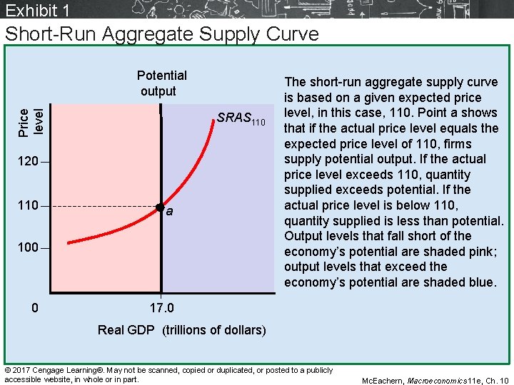
Exhibit 1 Short-Run Aggregate Supply Curve Price level Potential output SRAS 110 120 110 a 100 0 The short-run aggregate supply curve is based on a given expected price level, in this case, 110. Point a shows that if the actual price level equals the expected price level of 110, firms supply potential output. If the actual price level exceeds 110, quantity supplied exceeds potential. If the actual price level is below 110, quantity supplied is less than potential. Output levels that fall short of the economy’s potential are shaded pink; output levels that exceed the economy’s potential are shaded blue. 17. 0 Real GDP (trillions of dollars) © 2017 Cengage Learning®. May not be scanned, copied or duplicated, or posted to a publicly accessible website, in whole or in part. Mc. Eachern, Macroeconomics 11 e, Ch. 10

From the Short Run to the Long Run • Short-run equilibrium – Price level and real GDP when: – Aggregate demand curve intersects the short-run aggregate supply curve • Long run – Wage contracts and resource price agreements can be renegotiated – No surprises about the economy’s price level © 2017 Cengage Learning®. May not be scanned, copied or duplicated, or posted to a publicly accessible website, in whole or in part. Mc. Eachern, Macroeconomics 11 e, Ch. 10

From the Short Run to the Long Run • Expansionary gap – Amount by which actual output in the short run exceeds the economy’s potential output • The more that short run output exceeds the economy’s potential • The larger the expansionary gap • The greater the upward pressure on the price level © 2017 Cengage Learning®. May not be scanned, copied or duplicated, or posted to a publicly accessible website, in whole or in part. Mc. Eachern, Macroeconomics 11 e, Ch. 10

From the Short Run to the Long Run • Long run in macroeconomics – A period during which wage contracts and resource price agreements can be renegotiated – There are no surprises about the economy’s actual price level • Recessionary gap – Amount by which actual output in the short run falls short of the economy’s potential output © 2017 Cengage Learning®. May not be scanned, copied or duplicated, or posted to a publicly accessible website, in whole or in part. Mc. Eachern, Macroeconomics 11 e, Ch. 10

Closing an Expansionary Gap • AD greater than expected, short run: – Price level > expected – Output > potential – Unemployment < natural rate – Expansionary gap – Inflationary pressure © 2017 Cengage Learning®. May not be scanned, copied or duplicated, or posted to a publicly accessible website, in whole or in part. Mc. Eachern, Macroeconomics 11 e, Ch. 10

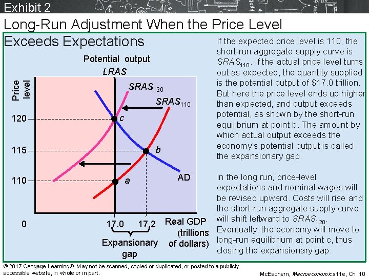
Exhibit 2 Long-Run Adjustment When the Price Level If the expected price level is 110, the Exceeds Expectations Price level Potential output LRAS 120 SRAS 110 c b 115 110 0 short-run aggregate supply curve is SRAS 110. If the actual price level turns out as expected, the quantity supplied is the potential output of $17. 0 trillion. But here the price level ends up higher than expected, and output exceeds potential, as shown by the short-run equilibrium at point b. The amount by which actual output exceeds the economy’s potential output is called the expansionary gap. In the long run, price-level expectations and nominal wages will be revised upward. Costs will rise and the short-run aggregate supply curve will shift leftward to SRAS 120. 17. 0 17. 2 Real GDP (trillions Eventually, the economy will move to Expansionary of dollars) long-run equilibrium at point c, thus closing the expansionary gap a AD © 2017 Cengage Learning®. May not be scanned, copied or duplicated, or posted to a publicly accessible website, in whole or in part. Mc. Eachern, Macroeconomics 11 e, Ch. 10

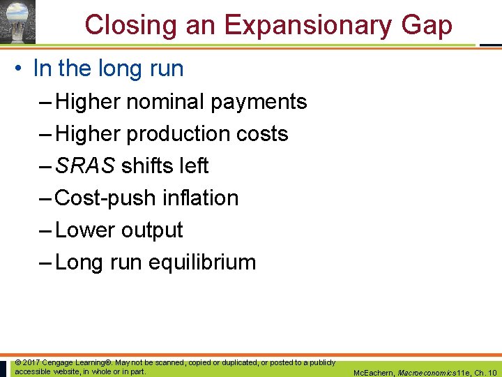
Closing an Expansionary Gap • In the long run – Higher nominal payments – Higher production costs – SRAS shifts left – Cost-push inflation – Lower output – Long run equilibrium © 2017 Cengage Learning®. May not be scanned, copied or duplicated, or posted to a publicly accessible website, in whole or in part. Mc. Eachern, Macroeconomics 11 e, Ch. 10

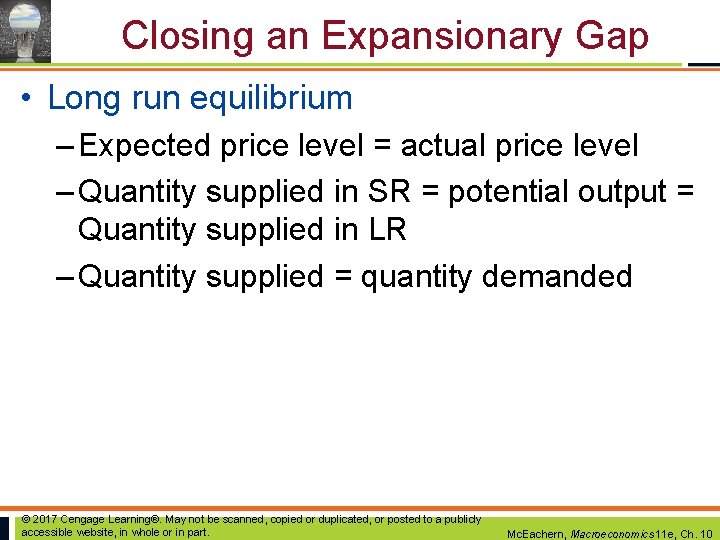
Closing an Expansionary Gap • Long run equilibrium – Expected price level = actual price level – Quantity supplied in SR = potential output = Quantity supplied in LR – Quantity supplied = quantity demanded © 2017 Cengage Learning®. May not be scanned, copied or duplicated, or posted to a publicly accessible website, in whole or in part. Mc. Eachern, Macroeconomics 11 e, Ch. 10

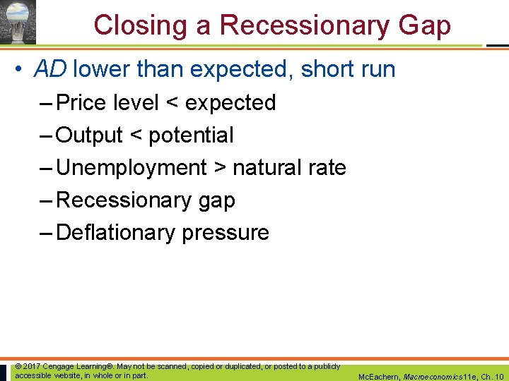
Closing a Recessionary Gap • AD lower than expected, short run – Price level < expected – Output < potential – Unemployment > natural rate – Recessionary gap – Deflationary pressure © 2017 Cengage Learning®. May not be scanned, copied or duplicated, or posted to a publicly accessible website, in whole or in part. Mc. Eachern, Macroeconomics 11 e, Ch. 10

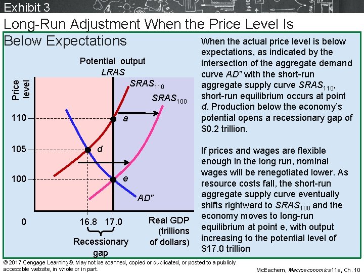
Exhibit 3 Price level Long-Run Adjustment When the Price Level Is When the actual price level is below Below Expectations Potential output LRAS SRAS 110 SRAS 100 110 105 a d e 100 AD″ 0 16. 8 17. 0 Recessionary gap Real GDP (trillions of dollars) expectations, as indicated by the intersection of the aggregate demand curve AD” with the short-run aggregate supply curve SRAS 110, short-run equilibrium occurs at point d. Production below the economy’s potential opens a recessionary gap of $0. 2 trillion. If prices and wages are flexible enough in the long run, nominal wages will be renegotiated lower. As resource costs fall, the short-run aggregate supply curve eventually shifts rightward to SRAS 100 and the economy moves to long-run equilibrium at point e, with output increasing to the potential level of $17. 0 trillion © 2017 Cengage Learning®. May not be scanned, copied or duplicated, or posted to a publicly accessible website, in whole or in part. Mc. Eachern, Macroeconomics 11 e, Ch. 10

Closing a Recessionary Gap • In the long run – Lower nominal wages – Lower cost of production – SRAS shifts right – Deflation – Greater output – Long run equilibrium © 2017 Cengage Learning®. May not be scanned, copied or duplicated, or posted to a publicly accessible website, in whole or in part. Mc. Eachern, Macroeconomics 11 e, Ch. 10

Long-Run Aggregate Supply Curve • Long-run aggregate supply curve, LRAS – Vertical line at the economy’s potential output – Aggregate supply when • There are no surprises about the price level • All resource contracts can be renegotiated • If wages and prices are flexible enough – The economy produces its potential output in the long run © 2017 Cengage Learning®. May not be scanned, copied or duplicated, or posted to a publicly accessible website, in whole or in part. Mc. Eachern, Macroeconomics 11 e, Ch. 10

Tracing Potential Output • Long-run aggregate supply curve, LRAS, depends on – Supply of resources in economy – Level of technology and know-how – Production incentives • Long-run equilibrium – Output = LRAS = potential output – Price level: depends on AD curve © 2017 Cengage Learning®. May not be scanned, copied or duplicated, or posted to a publicly accessible website, in whole or in part. Mc. Eachern, Macroeconomics 11 e, Ch. 10

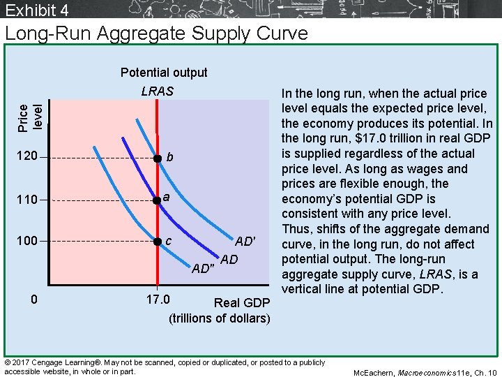
Exhibit 4 Long-Run Aggregate Supply Curve Price level Potential output LRAS 120 b 110 a 100 c AD″ 0 AD′ AD 17. 0 Real GDP (trillions of dollars) In the long run, when the actual price level equals the expected price level, the economy produces its potential. In the long run, $17. 0 trillion in real GDP is supplied regardless of the actual price level. As long as wages and prices are flexible enough, the economy’s potential GDP is consistent with any price level. Thus, shifts of the aggregate demand curve, in the long run, do not affect potential output. The long-run aggregate supply curve, LRAS, is a vertical line at potential GDP. © 2017 Cengage Learning®. May not be scanned, copied or duplicated, or posted to a publicly accessible website, in whole or in part. Mc. Eachern, Macroeconomics 11 e, Ch. 10

Wage Flexibility and Employment • Expansionary gap – Creates a labor shortage – Higher nominal wage – Higher price level • Recessionary gap – Nominal wages = “sticky” downward – Slow to close the gap © 2017 Cengage Learning®. May not be scanned, copied or duplicated, or posted to a publicly accessible website, in whole or in part. Mc. Eachern, Macroeconomics 11 e, Ch. 10

U. S. Output Gaps and Wage Flexibility • Recessionary gap – Resulting from a coordination failure • Workers and employers fail to achieve an outcome that all would prefer • “Sticky” wages downward – Why not shorter contracts? • Negotiating contracts – Costly and time consuming © 2017 Cengage Learning®. May not be scanned, copied or duplicated, or posted to a publicly accessible website, in whole or in part. Mc. Eachern, Macroeconomics 11 e, Ch. 10

U. S. Output Gaps and Wage Flexibility • Negotiating long-term contracts – Reduced cost of negotiation – Reduce frequency of strikes and lockouts • When demand is slack, layoffs instead of cutting nominal wages – Employers: lower wages hurts morale and reduce productivity – The incentive to accept a lower wage is reduced by the prospect of unemployment benefits © 2017 Cengage Learning®. May not be scanned, copied or duplicated, or posted to a publicly accessible website, in whole or in part. Mc. Eachern, Macroeconomics 11 e, Ch. 10

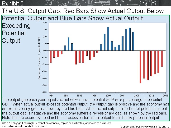
Exhibit 5 The U. S. Output Gap: Red Bars Show Actual Output Below Potential Output and Blue Bars Show Actual Output Exceeding Potential Output The output gap each year equals actual GDP minus potential GDP as a percentage of potential GDP. When actual output exceeds potential output, the output gap is positive and the economy has an expansionary gap, as shown by the blue bars. When actual output falls short of potential output, the output gap is negative and the economy suffers a recessionary gap, as shown by the red bars. Note that the economy need not be in recession for actual output to fall below potential output. © 2017 Cengage Learning®. May not be scanned, copied or duplicated, or posted to a publicly accessible website, in whole or in part. Mc. Eachern, Macroeconomics 11 e, Ch. 10

U. S. Output Gaps and Wage Flexibility • The Great Recession – High unemployment rates – Yet 9 in 10 workers still had jobs – Congress extended unemployment – Some states added to that extension – New York: some unemployed workers were eligible for up to 99 weeks of benefits © 2017 Cengage Learning®. May not be scanned, copied or duplicated, or posted to a publicly accessible website, in whole or in part. Mc. Eachern, Macroeconomics 11 e, Ch. 10

Aggregate Supply Increases • Aggregate supply increases, LRAS – Increased quantity and quality of labor • Size, composition, or quality of the labor force • Preferences for labor versus leisure – Increased quantity and quality of other resources • Capital stock, land – Institutional changes • Clearer patent and copyright laws © 2017 Cengage Learning®. May not be scanned, copied or duplicated, or posted to a publicly accessible website, in whole or in part. Mc. Eachern, Macroeconomics 11 e, Ch. 10

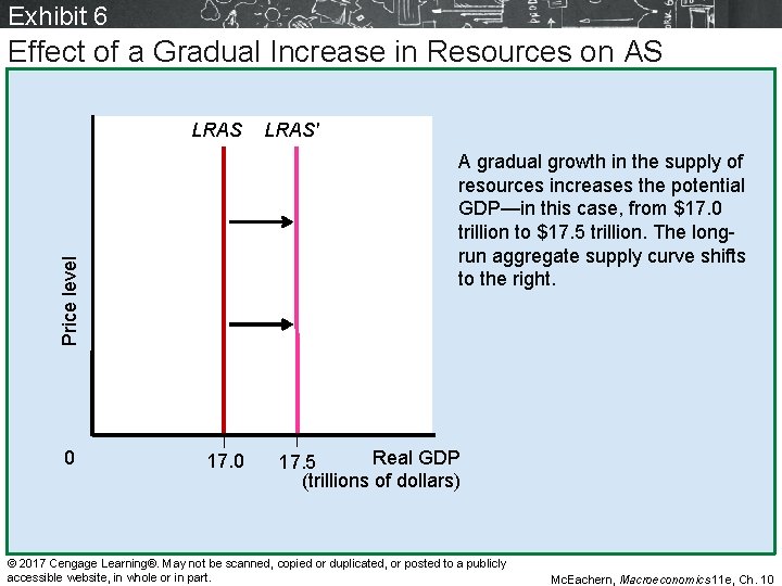
Exhibit 6 Effect of a Gradual Increase in Resources on AS LRAS A gradual growth in the supply of resources increases the potential GDP—in this case, from $17. 0 trillion to $17. 5 trillion. The longrun aggregate supply curve shifts to the right. Price level 0 LRAS′ 17. 0 Real GDP 17. 5 (trillions of dollars) © 2017 Cengage Learning®. May not be scanned, copied or duplicated, or posted to a publicly accessible website, in whole or in part. Mc. Eachern, Macroeconomics 11 e, Ch. 10

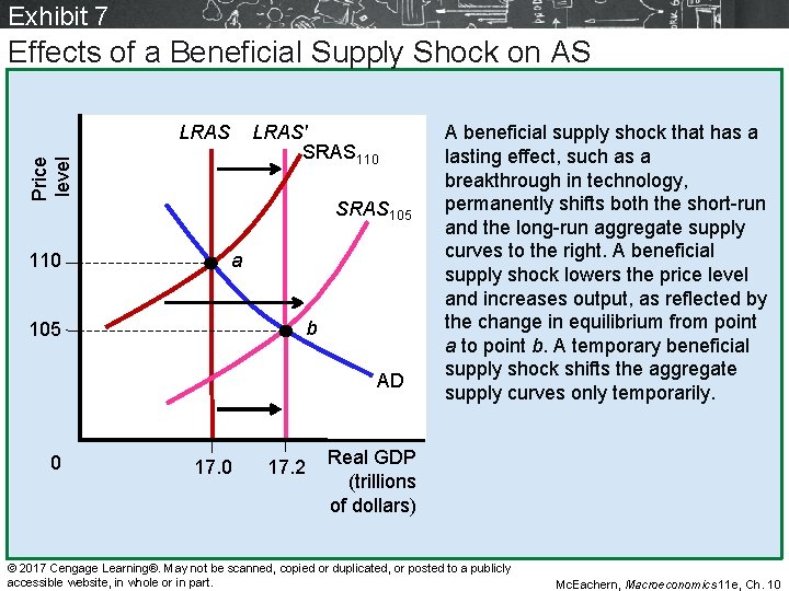
Aggregate Supply Increases • Supply shocks – Unexpected events that affect AS • Sometimes only temporarily • Beneficial supply shocks: increase AS • Abundant harvests • Technological breakthroughs • Discoveries of natural resources • Sudden changes in economic system that promote more production – Higher output and lower price level © 2017 Cengage Learning®. May not be scanned, copied or duplicated, or posted to a publicly accessible website, in whole or in part. Mc. Eachern, Macroeconomics 11 e, Ch. 10

Exhibit 7 Effects of a Beneficial Supply Shock on AS LRAS Price level LRAS′ SRAS 110 SRAS 105 a b 105 AD 0 17. 2 A beneficial supply shock that has a lasting effect, such as a breakthrough in technology, permanently shifts both the short-run and the long-run aggregate supply curves to the right. A beneficial supply shock lowers the price level and increases output, as reflected by the change in equilibrium from point a to point b. A temporary beneficial supply shock shifts the aggregate supply curves only temporarily. Real GDP (trillions of dollars) © 2017 Cengage Learning®. May not be scanned, copied or duplicated, or posted to a publicly accessible website, in whole or in part. Mc. Eachern, Macroeconomics 11 e, Ch. 10

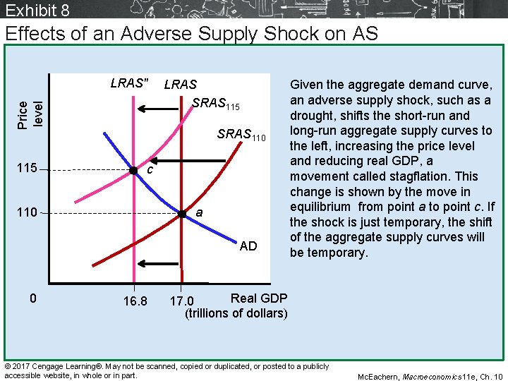
Aggregate Supply Decreases • Adverse supply shocks – Unexpected events that reduce aggregate supply, sometimes only temporarily • A drought • Overthrow of government • Terrorist attacks – Stagflation • Lower output • Higher price level © 2017 Cengage Learning®. May not be scanned, copied or duplicated, or posted to a publicly accessible website, in whole or in part. Mc. Eachern, Macroeconomics 11 e, Ch. 10

Exhibit 8 Effects of an Adverse Supply Shock on AS Price level LRAS″ 115 LRAS SRAS 115 SRAS 110 c 110 a AD 0 16. 8 Given the aggregate demand curve, an adverse supply shock, such as a drought, shifts the short-run and long-run aggregate supply curves to the left, increasing the price level and reducing real GDP, a movement called stagflation. This change is shown by the move in equilibrium from point a to point c. If the shock is just temporary, the shift of the aggregate supply curves will be temporary. Real GDP 17. 0 (trillions of dollars) © 2017 Cengage Learning®. May not be scanned, copied or duplicated, or posted to a publicly accessible website, in whole or in part. Mc. Eachern, Macroeconomics 11 e, Ch. 10

Hysteresis • Hysteresis – The theory that the natural rate of unemployment depends in part on the recent history of unemployment – A long period of high unemployment can increase the natural rate of unemployment • The longer the actual unemployment rate remains above what had been the natural rate, the more the natural rate itself increases © 2017 Cengage Learning®. May not be scanned, copied or duplicated, or posted to a publicly accessible website, in whole or in part. Mc. Eachern, Macroeconomics 11 e, Ch. 10

Hysteresis • Natural rate of unemployment has increased in Europe – Hysteresis – Generous unemployment benefits indefinitely, reducing the hardship of unemployment – Benefits are 60% to 80% of lost pay – Legislation: more difficult to layoff workers – Mandatory severance pay © 2017 Cengage Learning®. May not be scanned, copied or duplicated, or posted to a publicly accessible website, in whole or in part. Mc. Eachern, Macroeconomics 11 e, Ch. 10