Economic Fluctuations Junhui Qian Intermediate Macroeconomics Content Overview

Economic Fluctuations Junhui Qian Intermediate Macroeconomics

Content • • • Overview The IS-LM Models The AD-AS Model Keynes Theory Concluding Remarks Intermediate Macroeconomics

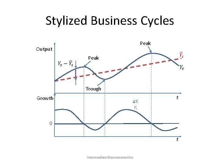
Business Cycle • The business cycle is the upward and downward movement of output around the long-term trend of output potential. • The business cycle is most often measured in terms of the growth rate of real GDP. Intermediate Macroeconomics

Stylized Business Cycles Peak Output Peak Trough Growth 0 Intermediate Macroeconomics

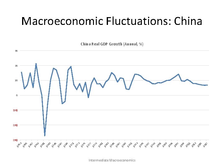
53 55 19 57 19 59 19 61 19 63 19 65 19 67 19 69 19 71 19 73 19 75 19 77 19 79 19 81 19 83 19 85 19 87 19 89 19 91 19 93 19 95 19 97 19 99 20 01 20 03 20 05 20 07 20 09 20 11 20 13 20 15 20 17 19 19 Macroeconomic Fluctuations: China Real GDP Growth (Annual, %) 30 20 10 0 (10) (20) (30) Intermediate Macroeconomics

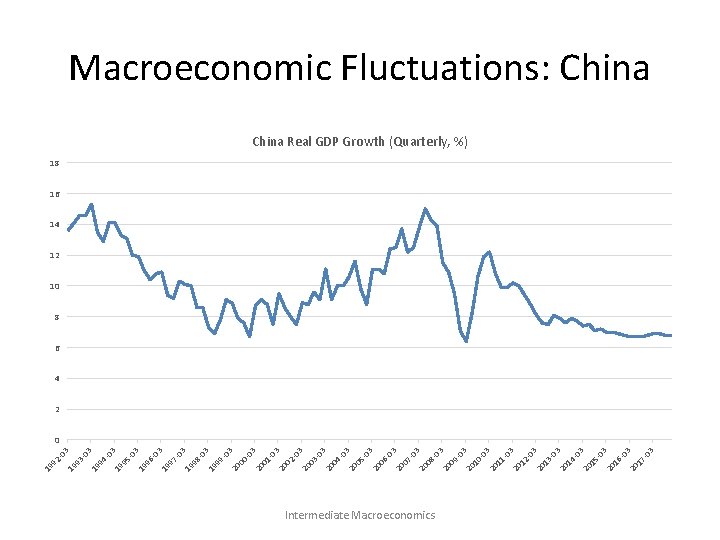
Intermediate Macroeconomics 3 -0 17 20 3 -0 16 20 3 -0 15 20 3 -0 14 20 3 -0 13 20 3 -0 12 20 3 -0 11 20 10 20 3 -0 09 20 08 20 3 -0 07 20 3 -0 06 20 3 -0 05 20 3 3 -0 -0 04 20 03 20 02 20 3 -0 01 20 00 20 3 -0 99 19 3 -0 98 19 3 -0 97 19 3 -0 96 19 95 19 3 -0 94 19 3 -0 93 19 92 19 Macroeconomic Fluctuations: China Real GDP Growth (Quarterly, %) 18 16 14 12 10 8 6 4 2 0

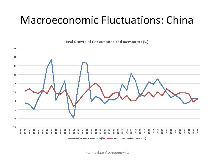
Macroeconomic Fluctuations: China Real Growth of Consumption and Investment (%) 35 30 25 20 15 10 5 0 Real Investment Growth (%) Real Consumption Growth (%) Intermediate Macroeconomics 2017 2018 2016 2015 2013 2014 2012 2011 2010 2009 2008 2007 2006 2005 2003 2004 2002 2001 2000 1999 1998 1997 1996 1995 1994 1992 1993 1991 1990 1988 1989 1987 1986 1985 1984 1983 1982 1981 1980 1979 -10 1978 -5

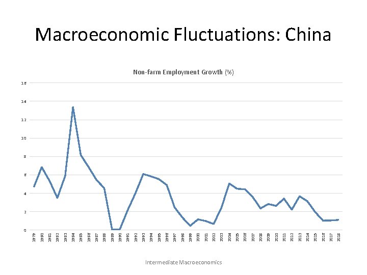
0 Intermediate Macroeconomics 2018 2017 2016 2015 2014 2013 2012 2011 2010 2009 2008 2007 2006 2005 2004 2003 2002 2001 2000 1999 1998 1997 1996 1995 1994 1993 1992 1991 1990 1989 1988 1987 1986 1985 1984 1983 1982 1981 1980 1979 Macroeconomic Fluctuations: China Non-farm Employment Growth (%) 16 14 12 10 8 6 4 2

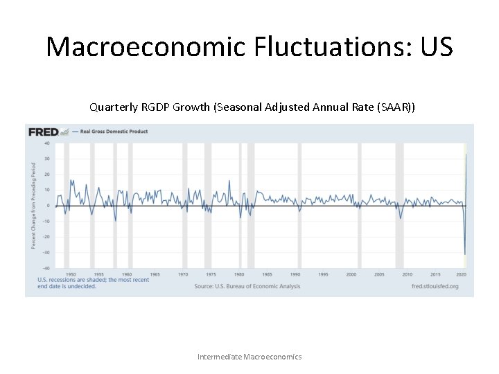
Macroeconomic Fluctuations: US Quarterly RGDP Growth (Seasonal Adjusted Annual Rate (SAAR)) Intermediate Macroeconomics

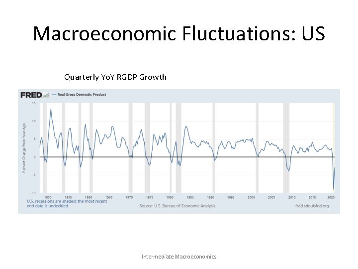
Macroeconomic Fluctuations: US Quarterly Yo. Y RGDP Growth Intermediate Macroeconomics

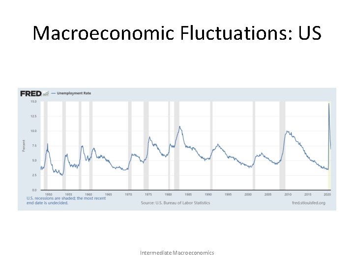
Macroeconomic Fluctuations: US Intermediate Macroeconomics

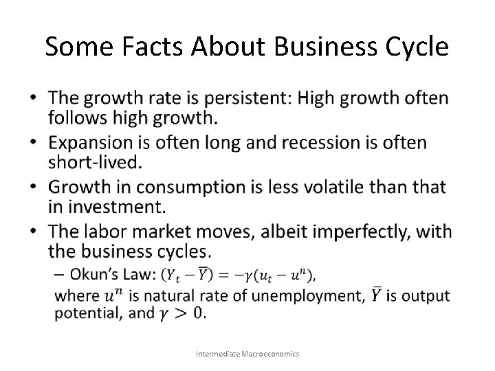
Some Facts About Business Cycle • Intermediate Macroeconomics

Identifying Recessions • In the United States, the official arbiter of when recessions begin and end is the NBER (National Bureau of Economic Research), a nonprofit economic research group. • The old rule of thumb: a recession is a period of at least two consecutive quarters of declining real GDP. • However, the NBER does not follow any fixed rule but use discretion in identifying recessions. Intermediate Macroeconomics

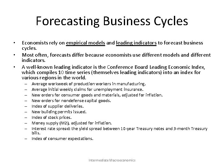
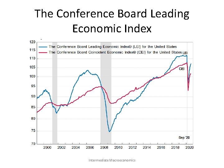
Forecasting Business Cycles • • • Economists rely on empirical models and leading indicators to forecast business cycles. Most often, forecasts differ because economists use different models and different indicators. A well-known leading indicator is the Conference Board Leading Economic Index, which compiles 10 time series (themselves leading indicators) into an index for various regions in the world. Average workweek of production workers in manufacturing. Average initial weekly claims for unemployment insurance. New orders for consumer goods and materials, adjusted for inflation. New orders for nondefense capital goods. Index of supplier deliveries. New building permits issued. Index of stock prices. Money supply (M 2), adjusted for inflation. Interest rate spread: the yield spread between 10 -year Treasury notes and 3 -month Treasury bills. – Index of consumer expectations. – – – – – Intermediate Macroeconomics

The Conference Board Leading Economic Index Intermediate Macroeconomics

Content • Overview • The IS-LM Models – The Keynesian Cross – The Sticky-Price Assumption – The IS-LM Model – Open Economy • The AD-AS Model • Keynes Theory • Concluding Remarks Intermediate Macroeconomics

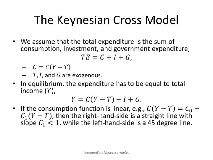
The Keynesian Cross Model • Intermediate Macroeconomics

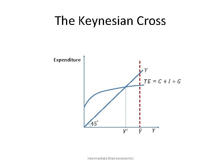
The Keynesian Cross Expenditure Intermediate Macroeconomics

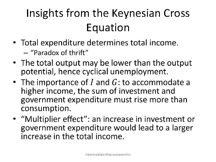
Insights from the Keynesian Cross Equation • Intermediate Macroeconomics

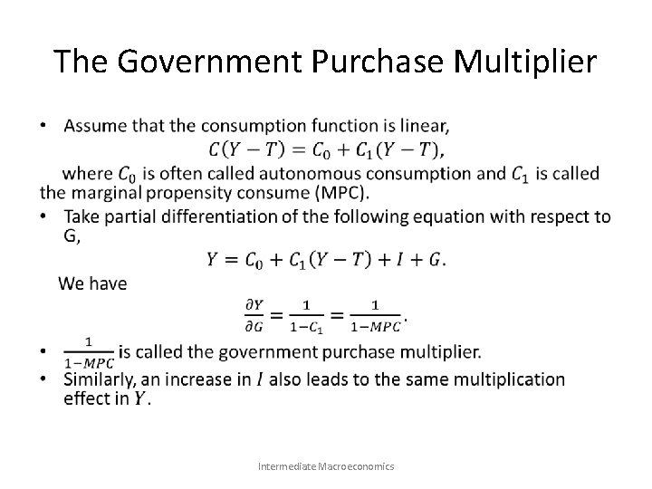
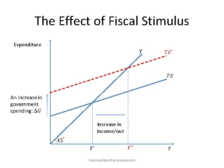
The Government Purchase Multiplier • Intermediate Macroeconomics

The Effect of Fiscal Stimulus Expenditure Increase in income/out Intermediate Macroeconomics

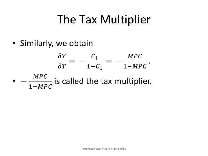
The Tax Multiplier • Intermediate Macroeconomics

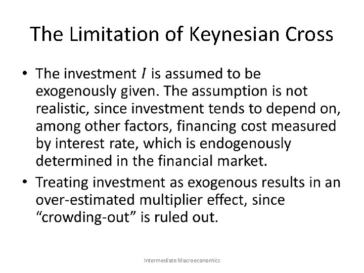
The Limitation of Keynesian Cross • Intermediate Macroeconomics

Content • Overview • The IS-LM Models – The Keynesian Cross – The Sticky-Price Assumption – The IS-LM Model – Open Economy • The AD-AS Model • Keynes Theory • Concluding Remarks Intermediate Macroeconomics

The Sticky-Price Assumption • The assumption says that prices are fixed in the short run. • The sticky-price assumption is crucial in the Keynesian models. – The price level can be treated as exogenous. – Markets do not automatically clear. – Classical dichotomy breaks down. Intermediate Macroeconomics

Time Horizons in Macroeconomics • Long run: Prices are flexible, responding to changes in supply or demand. • Short run: Many prices are “sticky” at some predetermined level. • In classical macroeconomic theory, output is determined by the supply side and changes in the demand side affects only prices. Hence price flexibility is a crucial assumption, which is only reasonable in the long run. • When prices are sticky, output and employment also depend on the demand. Intermediate Macroeconomics

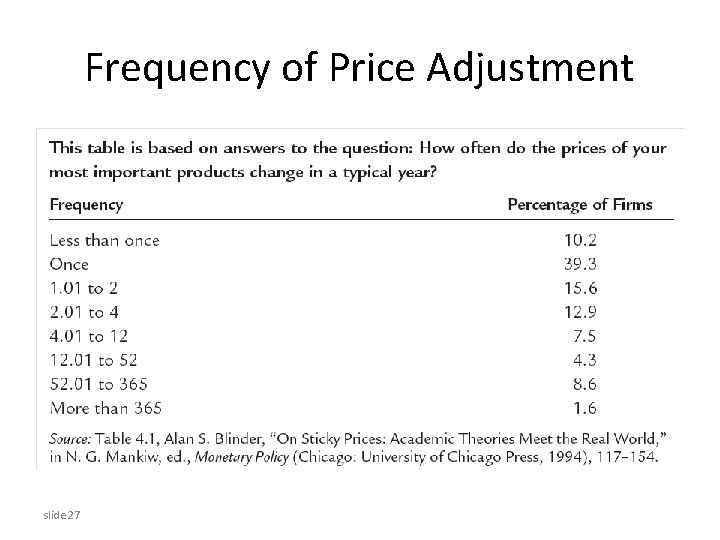
Frequency of Price Adjustment slide 27

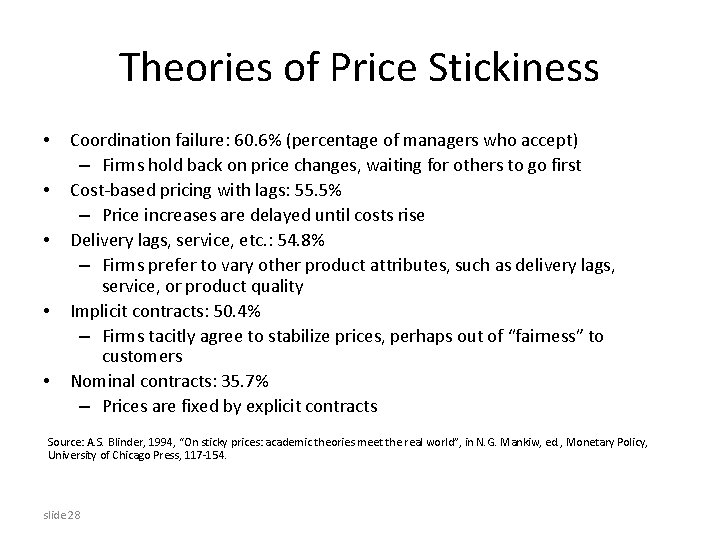
Theories of Price Stickiness • • • Coordination failure: 60. 6% (percentage of managers who accept) – Firms hold back on price changes, waiting for others to go first Cost-based pricing with lags: 55. 5% – Price increases are delayed until costs rise Delivery lags, service, etc. : 54. 8% – Firms prefer to vary other product attributes, such as delivery lags, service, or product quality Implicit contracts: 50. 4% – Firms tacitly agree to stabilize prices, perhaps out of “fairness” to customers Nominal contracts: 35. 7% – Prices are fixed by explicit contracts Source: A. S. Blinder, 1994, “On sticky prices: academic theories meet the real world”, in N. G. Mankiw, ed. , Monetary Policy, University of Chicago Press, 117 -154. slide 28

Content • Overview • The IS-LM Models – The Keynesian Cross – The Sticky-Price Assumption – The IS-LM Model – Open Economy • The AD-AS Model • Keynes Theory • Concluding Remarks Intermediate Macroeconomics

Overview of IS-LM • IS stands for “investment” and “saving”. • LM stands for “liquidity” and “money”. • The IS-LM model consists two equations that describe the financial market (IS, or equivalently the market for goods and services) and the money market (LM). • The IS-LM model is the leading interpretation of John Maynard Keynes’s theory, which was developed in the depth of the Great Depression. Intermediate Macroeconomics

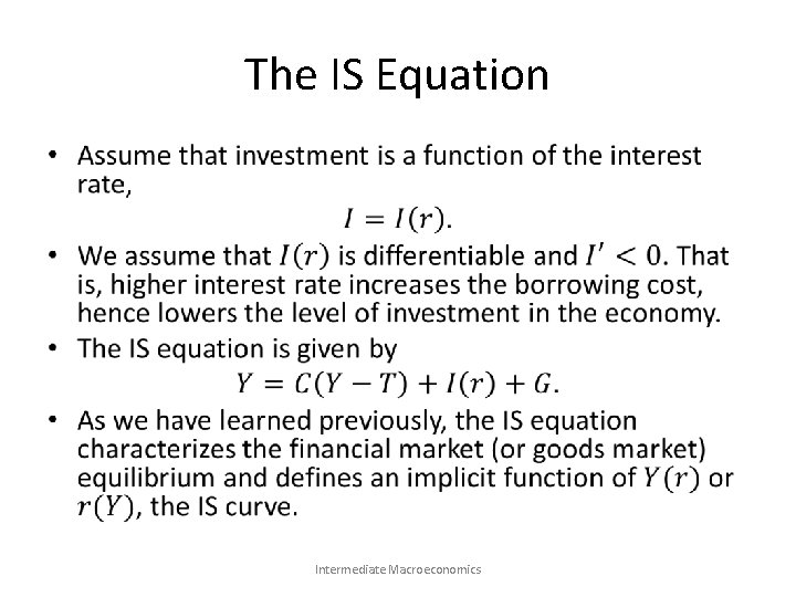
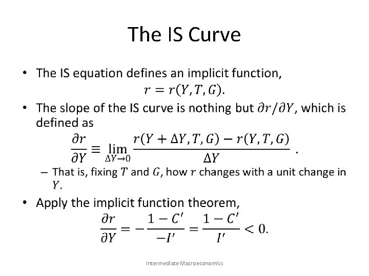
The IS Equation • Intermediate Macroeconomics

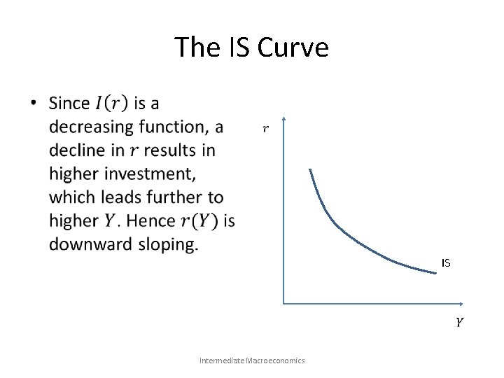
The IS Curve • IS Intermediate Macroeconomics

The IS Curve • Intermediate Macroeconomics

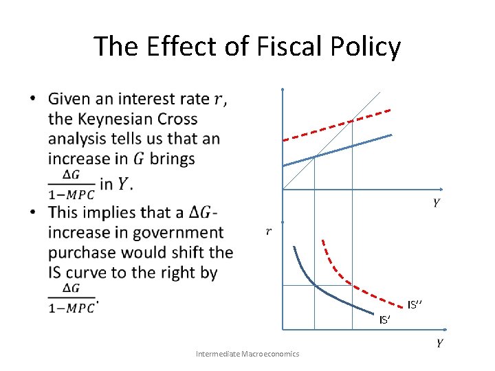
The Effect of Fiscal Policy • IS’’ IS’ Intermediate Macroeconomics

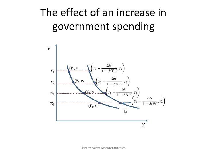
The effect of an increase in government spending IS Intermediate Macroeconomics

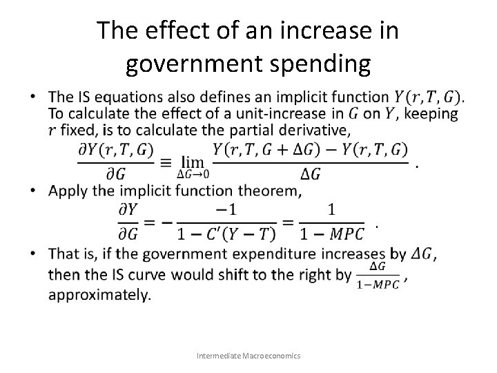
The effect of an increase in government spending • Intermediate Macroeconomics

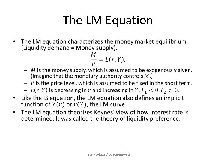
The LM Equation • Intermediate Macroeconomics

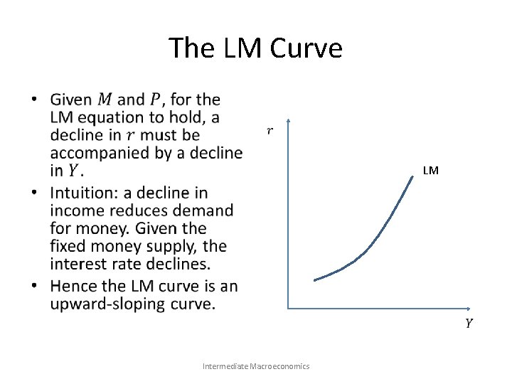
The LM Curve • LM Intermediate Macroeconomics

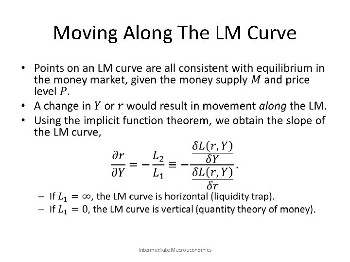
Moving Along The LM Curve • Intermediate Macroeconomics

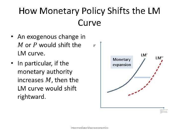
How Monetary Policy Shifts the LM Curve • Monetary expansion LM’’ Intermediate Macroeconomics

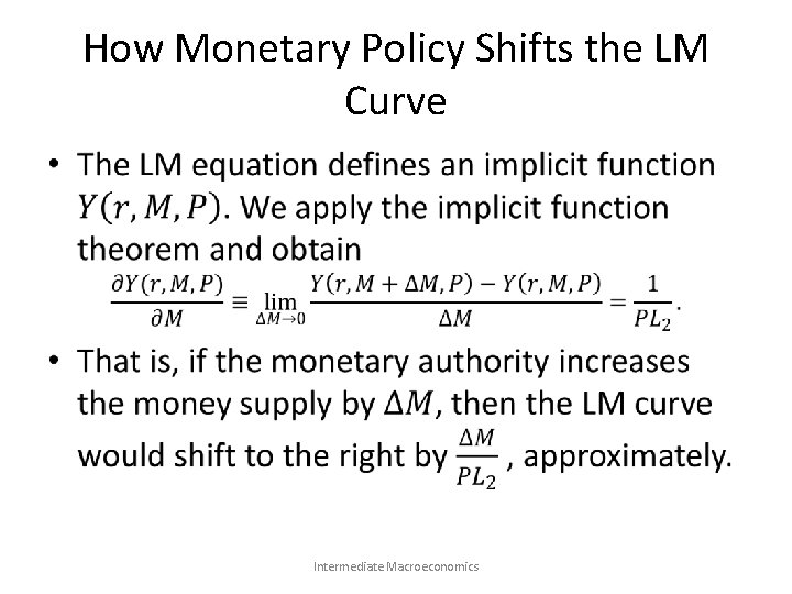
How Monetary Policy Shifts the LM Curve • Intermediate Macroeconomics

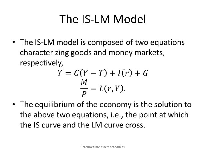
The IS-LM Model • Intermediate Macroeconomics

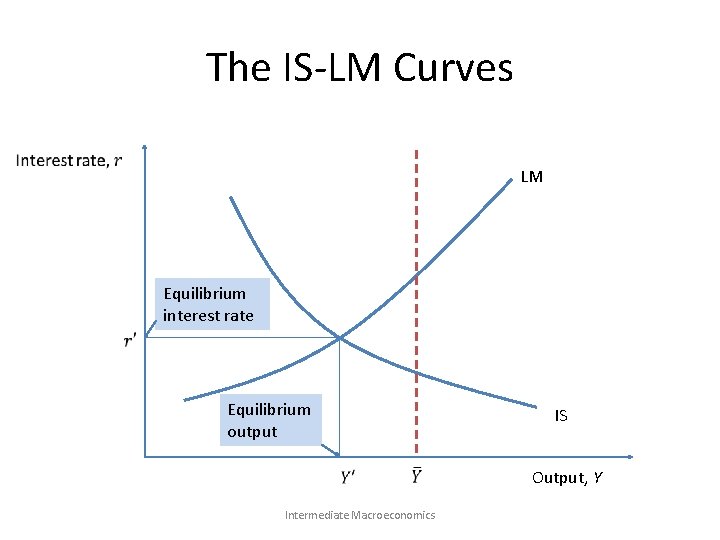
The IS-LM Curves LM Equilibrium interest rate Equilibrium output IS Intermediate Macroeconomics Output, Y

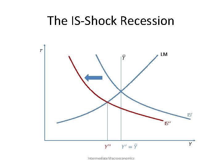
The IS-Shock Recession • As in the Keynesian Cross model, there is no reason to believe that the equilibrium output in the IS-LM stays at the level of output potential. Intermediate Macroeconomics

The IS-Shock Recession LM IS’’ Intermediate Macroeconomics Y

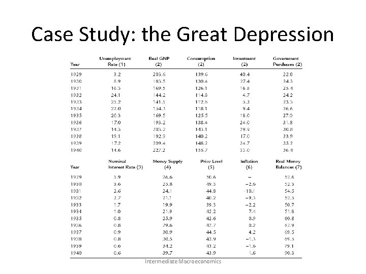
Case Study: the Great Depression Intermediate Macroeconomics

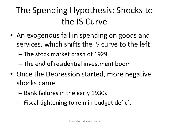
The Spending Hypothesis: Shocks to the IS Curve • An exogenous fall in spending on goods and services, which shifts the IS curve to the left. – The stock market crash of 1929 – The end of residential investment boom • Once the Depression started, more negative shocks came: – Bank failures in the early 1930 s – Fiscal tightening to rein in budget deficit. Intermediate Macroeconomics

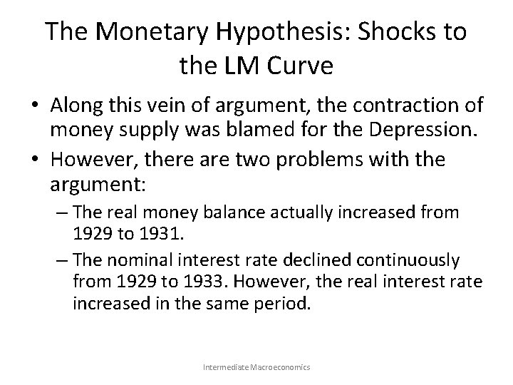
The Monetary Hypothesis: Shocks to the LM Curve • Along this vein of argument, the contraction of money supply was blamed for the Depression. • However, there are two problems with the argument: – The real money balance actually increased from 1929 to 1931. – The nominal interest rate declined continuously from 1929 to 1933. However, the real interest rate increased in the same period. Intermediate Macroeconomics

The Monetary Hypothesis: The Effects of Deflation • Deflation is defined as a fall in the general price level. • Deflation was thought to be good for the economy: – A fall in price expands the real money supply. – The Pigou effect: a fall in price brings about an increase in the purchasing power of the money balance held by households. The households feel wealthier and spend more, shifting the IS to the right. • However, deflation seems more effective in depressing income: – The debt-deflation theory – The role of expected deflation Intermediate Macroeconomics

The Debt-Deflation Theory • Assume that debtors (those who borrow money) have higher propensity to consume than creditors do. • Deflation increases debt burden, shifting purchasing power from debtors to creditors. • Under our assumption, the reduction of spending by the debtors is more than the increase of spending by the creditors. The net effect is a reduction of spending, shifting the IS curve to the left. Intermediate Macroeconomics

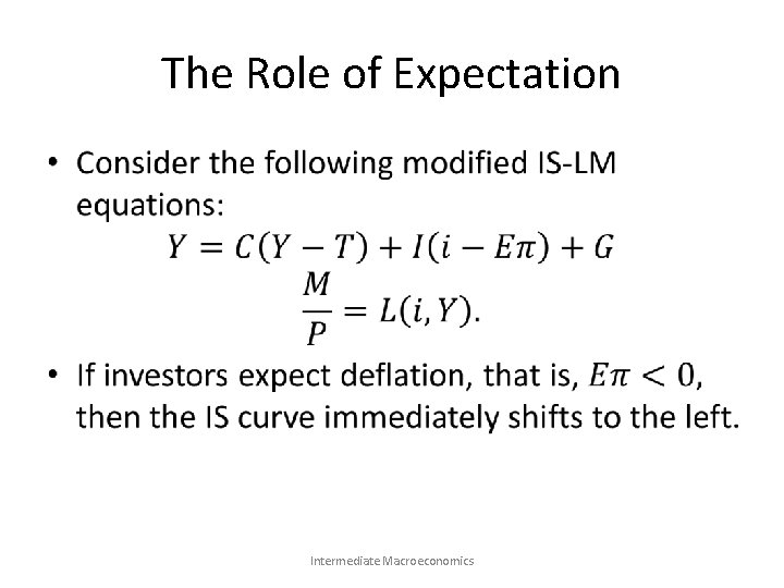
The Role of Expectation • Intermediate Macroeconomics

Policy Responses to Recessions • Policy makers may use fiscal, monetary, and both, to increase aggregate demand. • Fiscal stimulus – Increase in government purchasing – Tax reduction • Monetary stimulus • Combination of fiscal and monetary policies Intermediate Macroeconomics

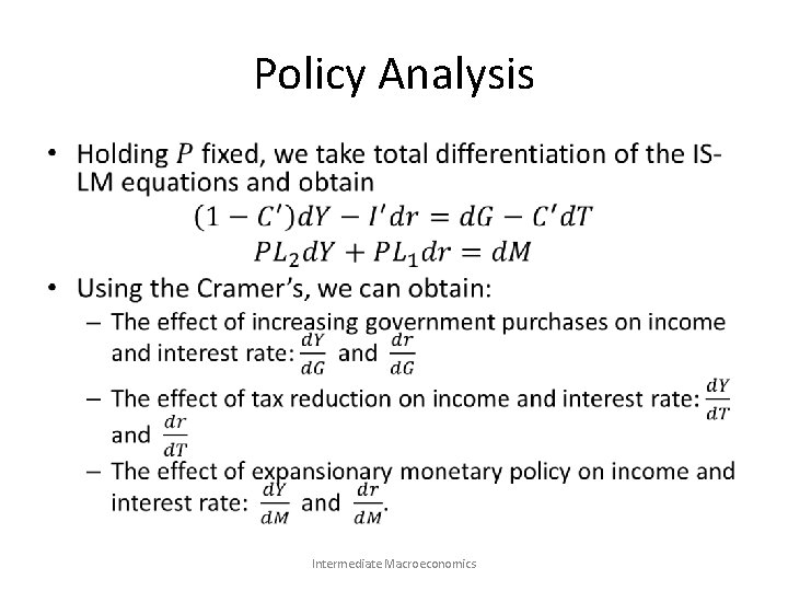
Policy Analysis • Intermediate Macroeconomics

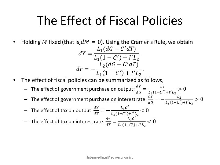
The Effect of Fiscal Policies • Intermediate Macroeconomics

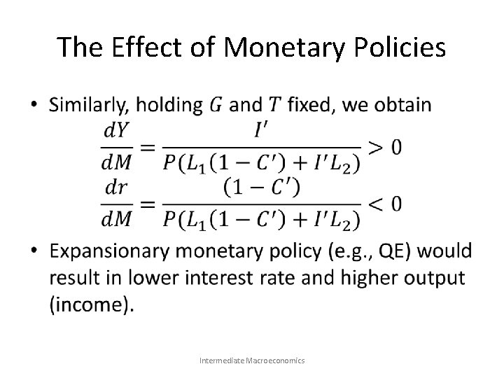
The Effect of Monetary Policies • Intermediate Macroeconomics

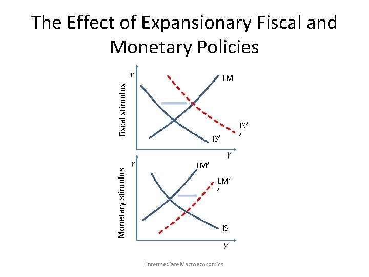
The Effect of Expansionary Fiscal and Monetary Policies Monetary stimulus Fiscal stimulus LM IS’ ’ IS’ LM’ ’ IS Intermediate Macroeconomics

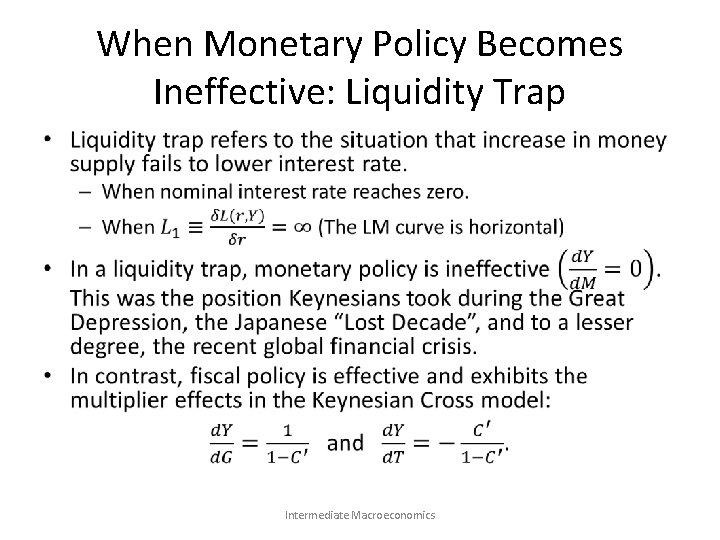
When Monetary Policy Becomes Ineffective: Liquidity Trap • Intermediate Macroeconomics

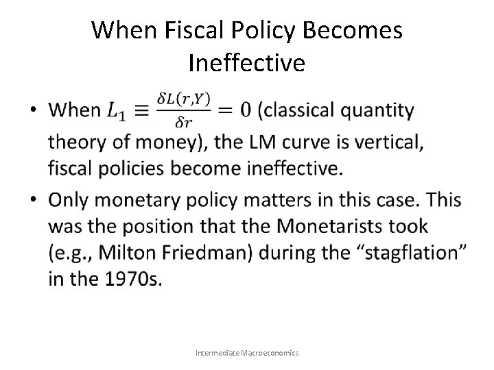
When Fiscal Policy Becomes Ineffective • Intermediate Macroeconomics

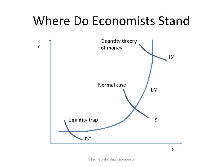
Where Do Economists Stand Quantity theory of money r IS’ Normal case Liquidity trap LM IS IS’’ Y Intermediate Macroeconomics

The Role of Interest Rate • Interest rate plays a central role in the IS-LM analysis of the economy. • In the normal case, – Expansionary monetary policy lowers interest rate, which encourages investment. – Fiscal stimulus drives up interest rate. This discourages investment and partly offsets the direct increase in output (income). • In a liquidity trap, – Expansionary monetary policy fails to lower interest rate. Hence no effect on output. • In the classical world, – Fiscal stimulus only drives up interest rate and completely “crowds out” investment. Intermediate Macroeconomics

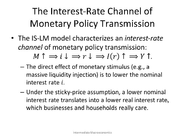
The Interest-Rate Channel of Monetary Policy Transmission • Intermediate Macroeconomics

Content • Overview • The IS-LM Models – – The Keynesian Cross The Sticky-Price Assumption The IS-LM Model Open Economy I. III. IV. Overview Small open economy with floating exchange rate Small open economy with fixed exchange rate Large open economy with floating exchange rate • The AD-AS Model • Keynes Theory • Concluding Remarks Intermediate Macroeconomics

Overview • We now consider open economies that trade with each other. • We shall study the effects of various shocks to exchange rate, money supply, interest rate, and output. • We assume that prices are sticky. Hence changes in real exchange rate is the same as nominal exchange rate. Intermediate Macroeconomics

Key Assumptions • The open economy, which allows trade and international finance. • Perfect capital mobility, which implies a common interest rate for the world. • Small economy, whose saving and investment does not affect the world interest rate. • Large economy, whose saving and investment does affect the world interest rate. Intermediate Macroeconomics

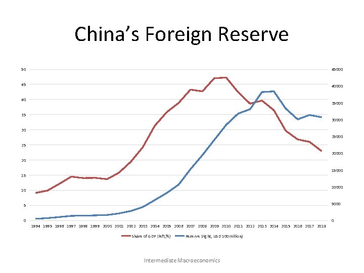
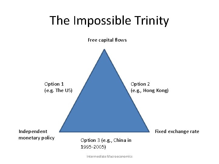
Fixed Exchange Rate • • • In a typical fixed exchange rate regime (e. g. , China from 1995 to 2005), the monetary authority stands ready to buy or sell the domestic currency at predetermined price (exchange rate). There are several other forms of exchange rate pegging: – Gold or silver standard (e. g. , Bretton Woods) – Monetary union (e. g. , Euro area) – “Dollarization” and currency boards (e. g. , Hong Kong, Argentina in 1990 s) Advantages of fixed exchange rate – Exchange rate stability – The “import” of responsible monetary policy from the advanced countries. Disadvantages of fixed exchange rate – Non-independence of monetary policy – To defend fixed rate against speculative attacks, the country has to accumulate a substantial amount of foreign exchange reserve. Intermediate Macroeconomics

China’s Foreign Reserve 50 45000 45 40000 40 35000 35 30000 30 25000 25 20000 20 15000 15 10000 10 5000 5 0 1994 1995 1996 1997 1998 1999 2000 2001 2002 2003 2004 2005 2006 2007 2008 2009 2010 2011 2012 2013 2014 2015 2016 2017 2018 Share of GDP (left, %) Reserve (right, USD 100 million) Intermediate Macroeconomics 0

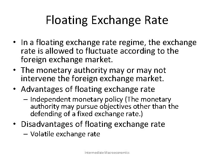
Floating Exchange Rate • In a floating exchange rate regime, the exchange rate is allowed to fluctuate according to the foreign exchange market. • The monetary authority may or may not intervene the foreign exchange market. • Advantages of floating exchange rate – Independent monetary policy (The monetary authority may pursue objectives other than the defending of a fixed exchange rate. ) • Disadvantages of floating exchange rate – Volatile exchange rate Intermediate Macroeconomics

The Impossible Trinity Free capital flows Option 1 (e. g. The US) Independent monetary policy Option 2 (e. g. , Hong Kong) Fixed exchange rate Option 3 (e. g. , China in 1995 -2005) Intermediate Macroeconomics

Content • Overview • The IS-LM Models – – The Keynesian Cross The Sticky-Price Assumption The IS-LM Model Open Economy I. III. IV. Overview Small open economy with floating exchange rate Small open economy with fixed exchange rate Large open economy with floating exchange rate • The AD-AS Model • Keynes Theory • Post-Keynesian Theories Intermediate Macroeconomics

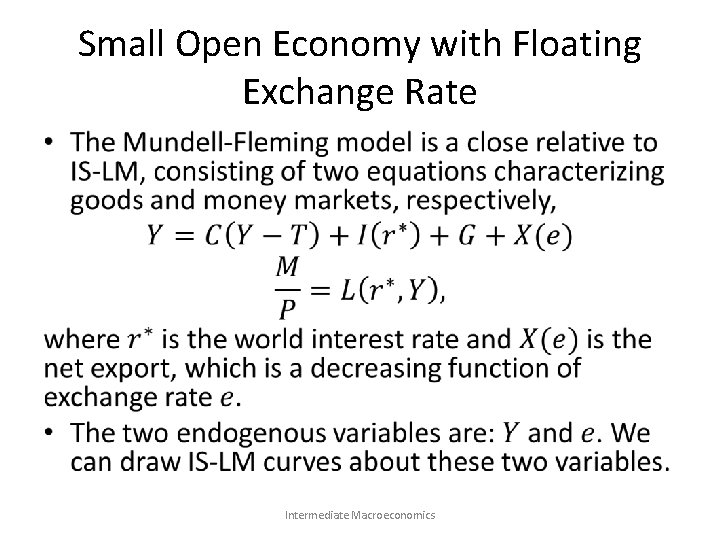
Small Open Economy with Floating Exchange Rate • Intermediate Macroeconomics

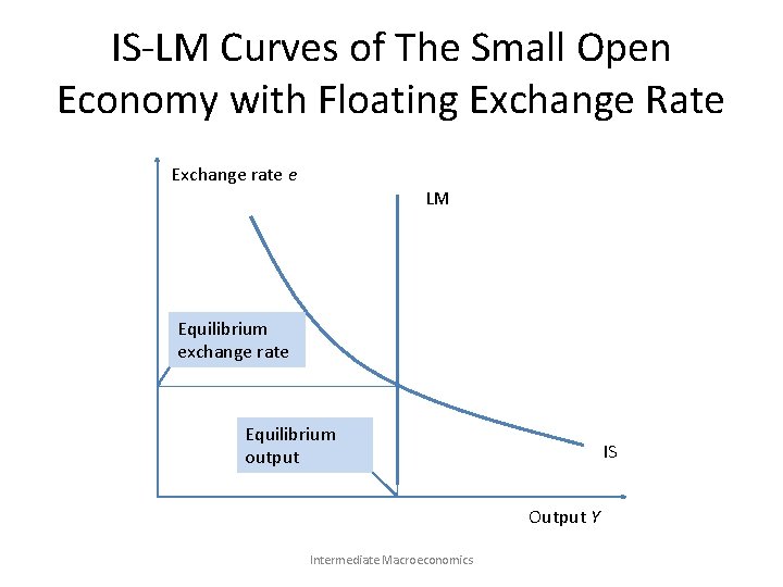
IS-LM Curves of The Small Open Economy with Floating Exchange Rate Exchange rate e LM Equilibrium exchange rate Equilibrium output IS Output Y Intermediate Macroeconomics

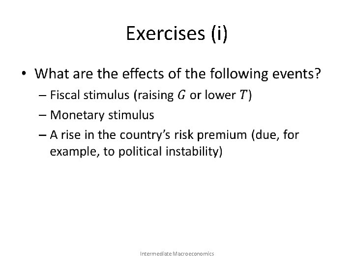
Exercises (i) • Intermediate Macroeconomics

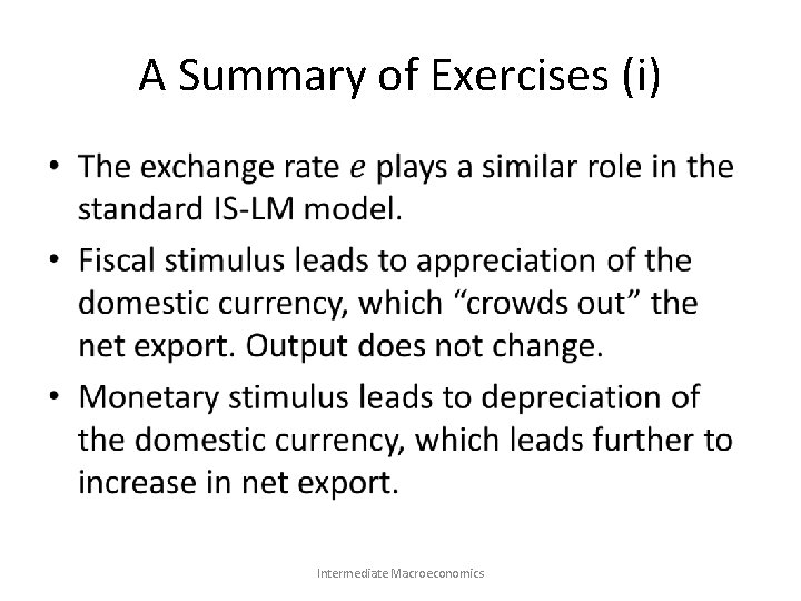
A Summary of Exercises (i) • Intermediate Macroeconomics

Content • Overview • The IS-LM Models – – The Keynesian Cross The Sticky-Price Assumption The IS-LM Model Open Economy I. III. IV. Overview Small open economy with floating exchange rate Small open economy with fixed exchange rate Large open economy with floating exchange rate • The AD-AS Model • Keynes Theory • Concluding Remarks Intermediate Macroeconomics

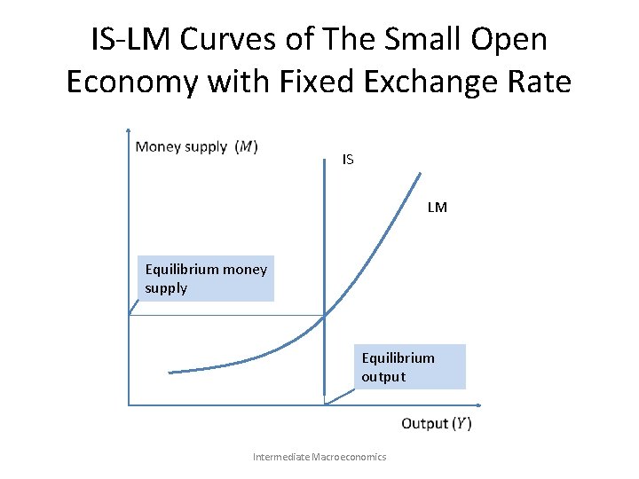
Small Open Economy with Fixed Exchange Rate • Under the fixed exchange regime, the monetary authority stands ready to buy or sell the domestic currency at pre-determined price (exchange rate). • When the monetary authority buys the domestic currency with a foreign currency, the monetary authority tightens the money supply. • When the monetary authority sells the domestic currency for a foreign currency, the monetary authority expands the money supply. • If the exchange rate is fixed, the money supply is endogenous. Intermediate Macroeconomics

The Role of Foreign Exchange Reserve • To conduct the intervention, the monetary authority needs a solid foreign currency reserve for the defense of the fixed exchange rate. • Under the fixed exchange rate regime, net capital outflow = net private capital outflow + increase in foreign reserve. • The increase in foreign reserve corresponds to increase in domestic money supply. Intermediate Macroeconomics

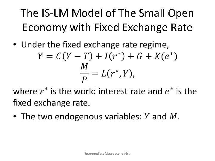
The IS-LM Model of The Small Open Economy with Fixed Exchange Rate • Intermediate Macroeconomics

IS-LM Curves of The Small Open Economy with Fixed Exchange Rate IS LM Equilibrium money supply Equilibrium output Intermediate Macroeconomics

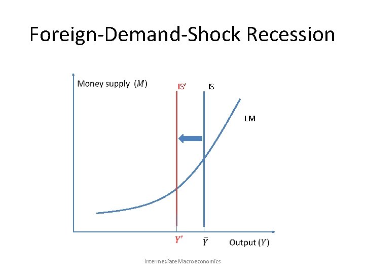
Foreign-Demand-Shock Recession IS’ IS LM Intermediate Macroeconomics

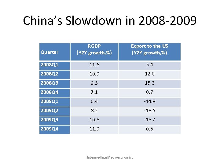
China’s Slowdown in 2008 -2009 • China’s GDP in 2007 was about 26% of the US GDP. • The “crawling peg” of RMB to USD: although the RMB exchange rate was no longer pegged to USD, it was still rigid and was allowed to appreciate very slowly. • As the financial crisis hit the US, the US demand for Chinese goods took a nosedive, resulting in China’s slowdown. Intermediate Macroeconomics

China’s Slowdown in 2008 -2009 Quarter RGDP (Y 2 Y growth, %) Export to the US (Y 2 Y growth, %) 2008 Q 1 11. 5 5. 4 2008 Q 2 10. 9 12. 0 2008 Q 3 9. 5 15. 3 2008 Q 4 7. 1 0. 7 2009 Q 1 6. 4 -14. 8 2009 Q 2 8. 2 -18. 5 2009 Q 3 10. 6 -16. 7 2009 Q 4 11. 9 0. 6 Intermediate Macroeconomics

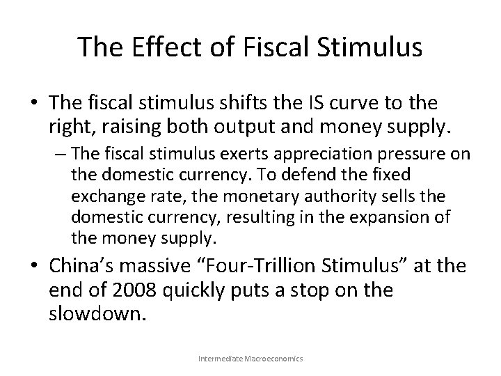
The Effect of Fiscal Stimulus • The fiscal stimulus shifts the IS curve to the right, raising both output and money supply. – The fiscal stimulus exerts appreciation pressure on the domestic currency. To defend the fixed exchange rate, the monetary authority sells the domestic currency, resulting in the expansion of the money supply. • China’s massive “Four-Trillion Stimulus” at the end of 2008 quickly puts a stop on the slowdown. Intermediate Macroeconomics

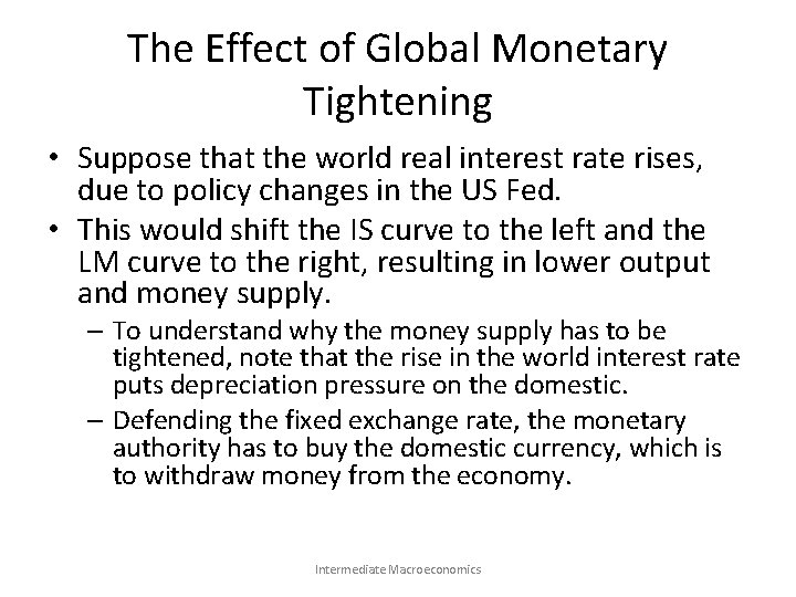
The Effect of Global Monetary Tightening • Suppose that the world real interest rate rises, due to policy changes in the US Fed. • This would shift the IS curve to the left and the LM curve to the right, resulting in lower output and money supply. – To understand why the money supply has to be tightened, note that the rise in the world interest rate puts depreciation pressure on the domestic. – Defending the fixed exchange rate, the monetary authority has to buy the domestic currency, which is to withdraw money from the economy. Intermediate Macroeconomics

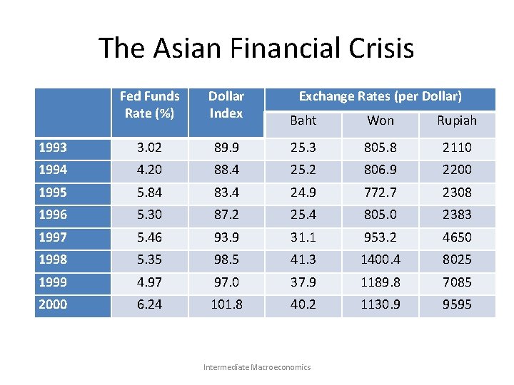
The Asian Financial Crisis Fed Funds Rate (%) Dollar Index 1993 3. 02 1994 Exchange Rates (per Dollar) Baht Won Rupiah 89. 9 25. 3 805. 8 2110 4. 20 88. 4 25. 2 806. 9 2200 1995 5. 84 83. 4 24. 9 772. 7 2308 1996 5. 30 87. 2 25. 4 805. 0 2383 1997 5. 46 93. 9 31. 1 953. 2 4650 1998 5. 35 98. 5 41. 3 1400. 4 8025 1999 4. 97 97. 0 37. 9 1189. 8 7085 2000 6. 24 101. 8 40. 2 1130. 9 9595 Intermediate Macroeconomics

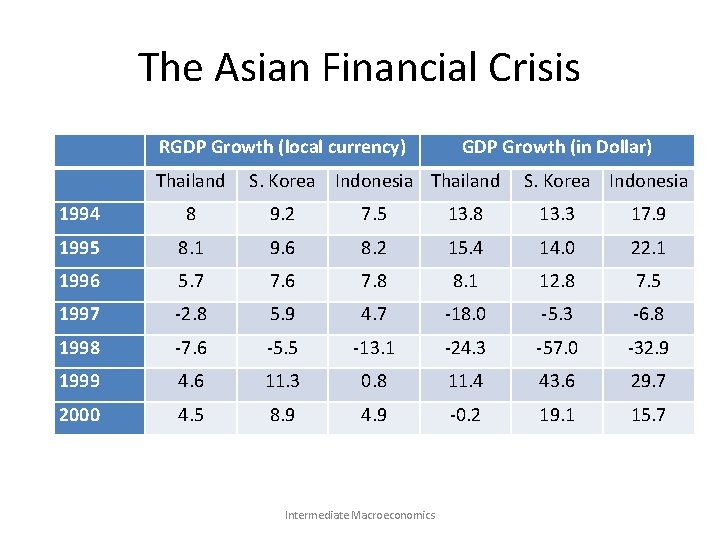
The Asian Financial Crisis RGDP Growth (local currency) Thailand GDP Growth (in Dollar) S. Korea Indonesia Thailand S. Korea Indonesia 1994 8 9. 2 7. 5 13. 8 13. 3 17. 9 1995 8. 1 9. 6 8. 2 15. 4 14. 0 22. 1 1996 5. 7 7. 6 7. 8 8. 1 12. 8 7. 5 1997 -2. 8 5. 9 4. 7 -18. 0 -5. 3 -6. 8 1998 -7. 6 -5. 5 -13. 1 -24. 3 -57. 0 -32. 9 1999 4. 6 11. 3 0. 8 11. 4 43. 6 29. 7 2000 4. 5 8. 9 4. 9 -0. 2 19. 1 15. 7 Intermediate Macroeconomics

Content • Overview • The IS-LM Models – – The Keynesian Cross The Sticky-Price Assumption The IS-LM Model Open Economy I. III. IV. Overview Small open economy with floating exchange rate Small open economy with fixed exchange rate Large open economy with floating exchange rate • The AD-AS Model • Keynes Theory • Concluding Remarks Intermediate Macroeconomics

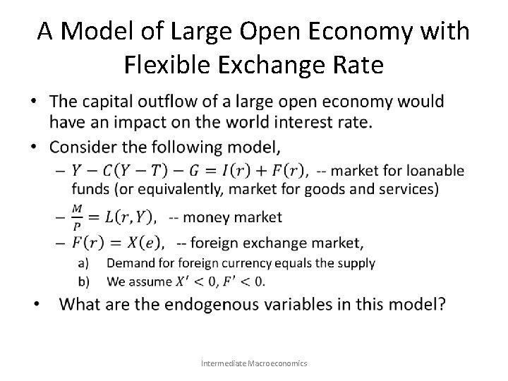
A Model of Large Open Economy with Flexible Exchange Rate • Intermediate Macroeconomics

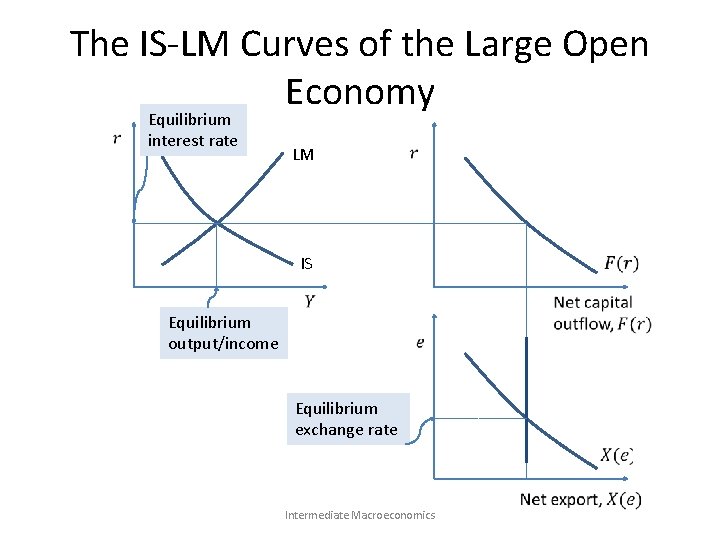
The IS-LM Curves of the Large Open Economy Equilibrium interest rate LM IS Equilibrium output/income Equilibrium exchange rate Intermediate Macroeconomics

Exercises (iii) • What would be the effects of the following changes? – Fiscal stimulus – Monetary stimulus – A protectionist policy shock (e. g. , an import tax) Intermediate Macroeconomics

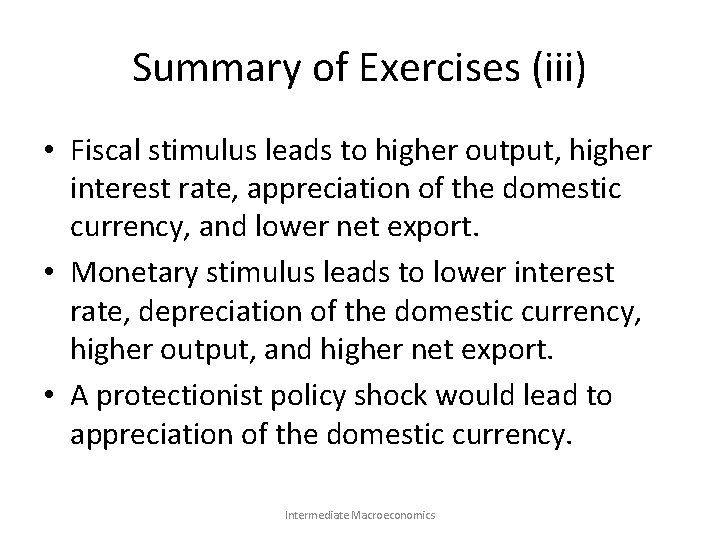
Summary of Exercises (iii) • Fiscal stimulus leads to higher output, higher interest rate, appreciation of the domestic currency, and lower net export. • Monetary stimulus leads to lower interest rate, depreciation of the domestic currency, higher output, and higher net export. • A protectionist policy shock would lead to appreciation of the domestic currency. Intermediate Macroeconomics

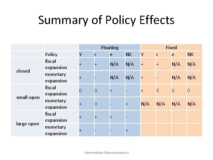
Summary of Policy Effects 　 Policy fiscal expansion 　closed monetary expansion fiscal expansion 　small open monetary expansion fiscal expansion 　large open monetary expansion 　 Y Floating r e NX Y r + + N/A N/A + - N/A N/A 0 0 + - + 0 0 0 + 0 - + N/A N/A + + + - - + 　 Intermediate Macroeconomics Fixed e NX

Content • Overview • The IS-LM Models • The AD-AS Model – Aggregate Demand – Aggregate Supply – Phillips Curve – Dynamic AD-AS Model • Keynes Theory • Concluding Remarks Intermediate Macroeconomics

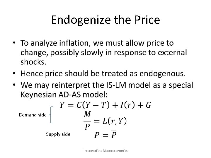
Endogenize the Price • Demand side Supply side Intermediate Macroeconomics

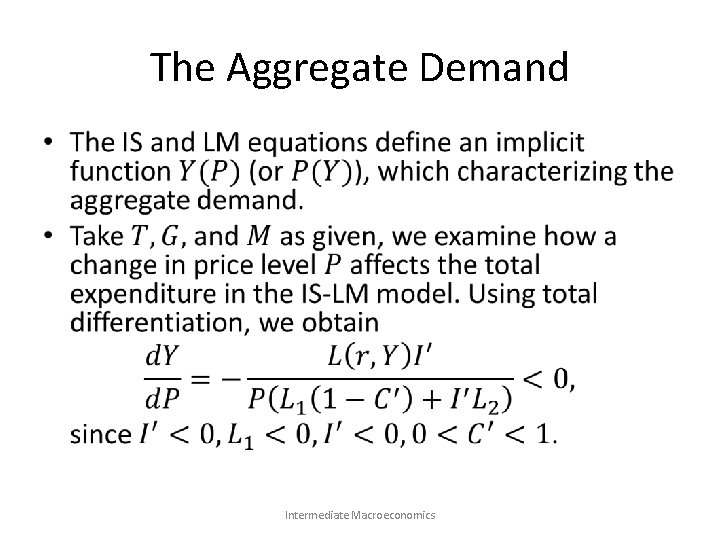
The Aggregate Demand • Intermediate Macroeconomics

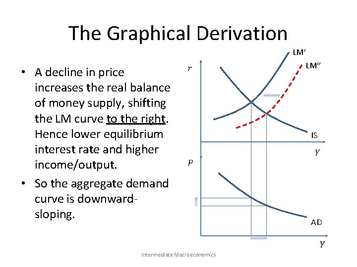
The Graphical Derivation • A decline in price increases the real balance of money supply, shifting the LM curve to the right. Hence lower equilibrium interest rate and higher income/output. • So the aggregate demand curve is downwardsloping. LM’’ IS AD Intermediate Macroeconomics

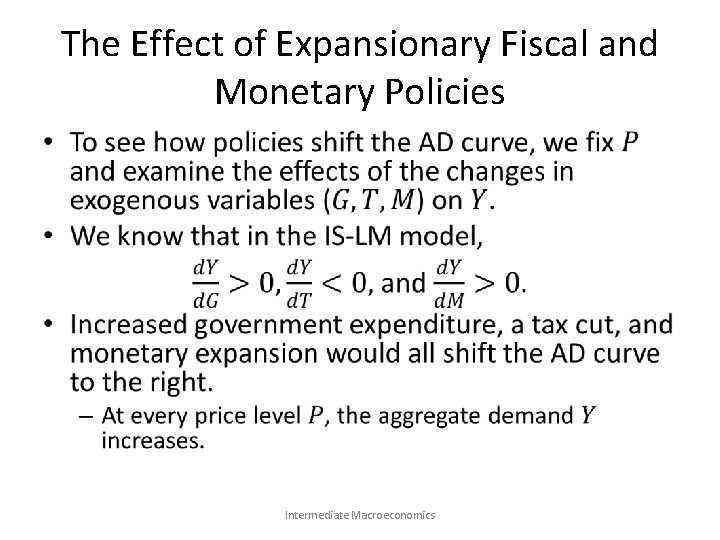
The Effect of Expansionary Fiscal and Monetary Policies • Intermediate Macroeconomics

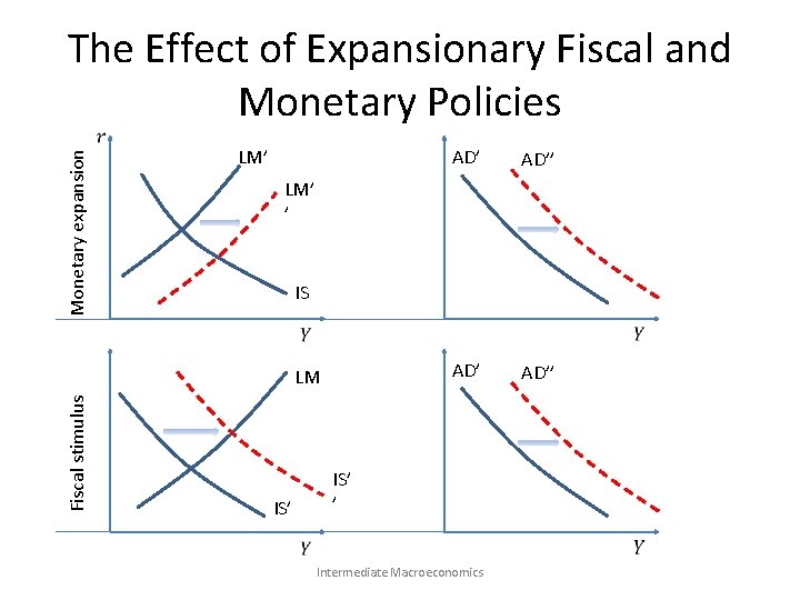
The Effect of Expansionary Fiscal and Monetary Policies Monetary expansion LM’ AD’’ LM’ ’ IS AD’ Fiscal stimulus LM AD’’ IS’ Intermediate Macroeconomics

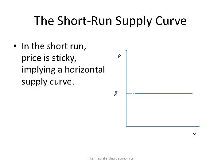
The Short-Run Supply Curve • In the short run, price is sticky, implying a horizontal supply curve. P Y Intermediate Macroeconomics

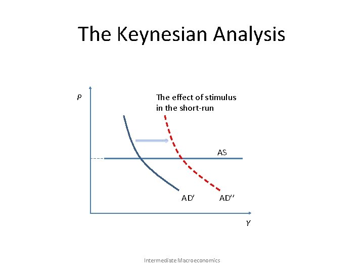
The Keynesian Analysis P The effect of stimulus in the short-run AS AD’’ Y Intermediate Macroeconomics

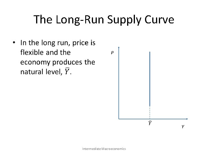
The Long-Run Supply Curve • P Intermediate Macroeconomics Y

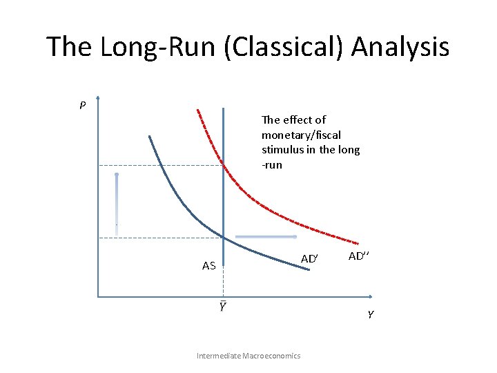
The Long-Run (Classical) Analysis P The effect of monetary/fiscal stimulus in the long -run AS Intermediate Macroeconomics AD’’ Y

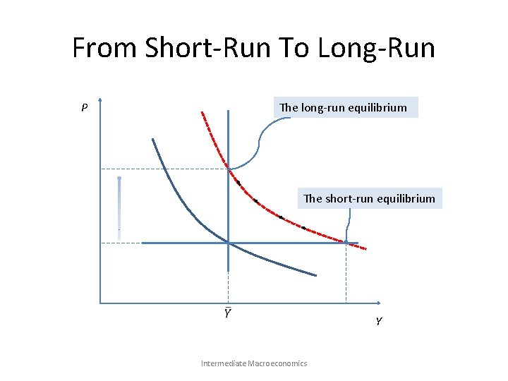
From Short-Run To Long-Run The long-run equilibrium P The short-run equilibrium Intermediate Macroeconomics Y

Stabilization Policy • The government, as either the monetary authority or the biggest spender, is able to stabilize an economy that, under constant shocks, deviate from long-run natural levels of output and employment. • A shock to the economy may come from the demand side or the supply side. Intermediate Macroeconomics

Shocks to Aggregate Demand • Intermediate Macroeconomics

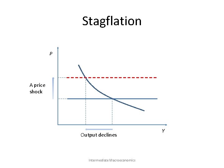
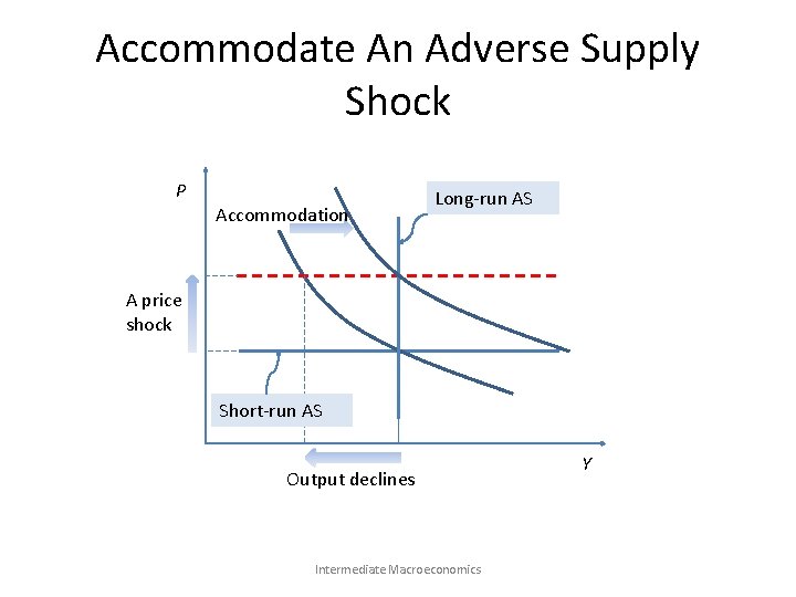
Shocks to Aggregate Supply • A supply shock changes the factor prices or the technology. • A supply shock is invariably associated with a change in price. Hence we often call it price shock. • Examples of adverse supply shocks: – A severe drought – A new environmental protection law – An increase in labor unrest or union aggressiveness – The formation of an international oil cartel Intermediate Macroeconomics

Stagflation P A price shock Output declines Intermediate Macroeconomics Y

Accommodate An Adverse Supply Shock P Accommodation Long-run AS A price shock Short-run AS Output declines Intermediate Macroeconomics Y

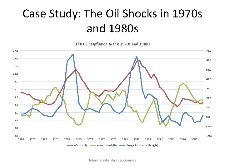
Case Study: The Oil Shocks in 1970 s and 1980 s The US Stagflation in the 1970 s and 1980 s 17. 0 70. 0 15. 0 60. 0 13. 0 50. 0 11. 0 40. 0 9. 0 7. 0 30. 0 5. 0 20. 0 3. 0 10. 0 1. 0 0. 0 -10. 0 -3. 0 -5. 0 1971 1972 1973 1974 1975 Inflation (%) 1976 1977 1978 RGDP Growth (%) 1979 1980 1981 1982 Change in Oil Price (%, right) Intermediate Macroeconomics 1983 1984 1985 -20. 0

Content • Overview • The IS-LM Models • The AD-AS Model – Aggregate Demand – Aggregate Supply – Phillips Curve – Dynamic AD-AS Model • Keynes Theory • Concluding Remarks Intermediate Macroeconomics

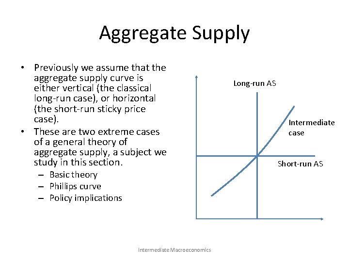
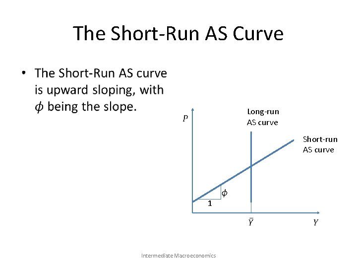
Aggregate Supply • Previously we assume that the aggregate supply curve is either vertical (the classical long-run case), or horizontal (the short-run sticky price case). • These are two extreme cases of a general theory of aggregate supply, a subject we study in this section. – Basic theory – Phillips curve – Policy implications Intermediate Macroeconomics Long-run AS Intermediate case Short-run AS

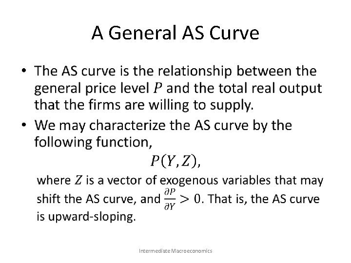
A General AS Curve • Intermediate Macroeconomics

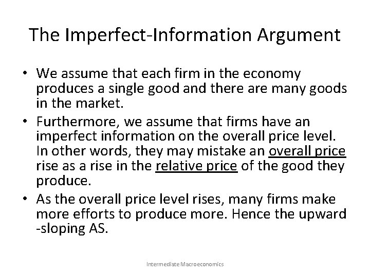
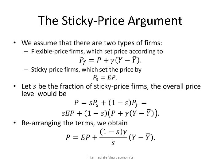
The Imperfect-Information Argument • We assume that each firm in the economy produces a single good and there are many goods in the market. • Furthermore, we assume that firms have an imperfect information on the overall price level. In other words, they may mistake an overall price rise as a rise in the relative price of the good they produce. • As the overall price level rises, many firms make more efforts to produce more. Hence the upward -sloping AS. Intermediate Macroeconomics

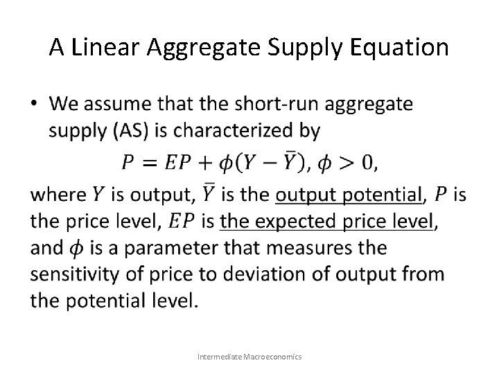
A Linear Aggregate Supply Equation • Intermediate Macroeconomics

The Short-Run AS Curve • Long-run AS curve Short-run AS curve 1 Intermediate Macroeconomics

The Sticky-Price Argument • Intermediate Macroeconomics

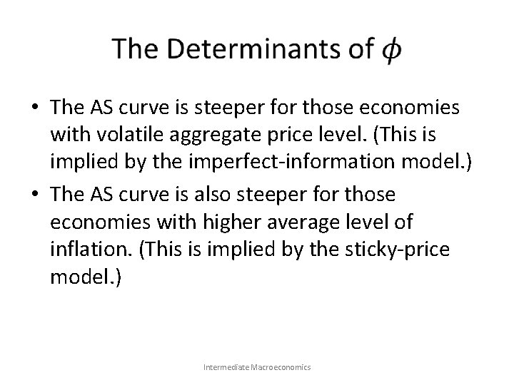
• The AS curve is steeper for those economies with volatile aggregate price level. (This is implied by the imperfect-information model. ) • The AS curve is also steeper for those economies with higher average level of inflation. (This is implied by the sticky-price model. ) Intermediate Macroeconomics

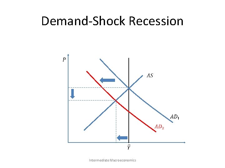
Demand-Shock Recession Intermediate Macroeconomics

Demand-Shock Recession • If there is a negative shock to the aggregate demand, e. g. , reduced investment sentiment, then the economy would enter a recession. – Output declines, unemployment rises, and price declines (deflation). • Recall that deflation may further reduce aggregate demand. – Transfer wealth from debtors to creditors, who generally have less MPC. – The deflation expectation raises the real interest rate, further reducing investment. Intermediate Macroeconomics

Policy Response to Demand-Shock Recessions • In normal cases, both fiscal and monetary policies may be employed to increase aggregate demand. • However, if the recession is deep and there is widespread panic (e. g. , liquidity trap), monetary policy alone may not work. • Even a tax cut may not work since people may choose to save the extra money. • Under such circumstances, government expenditure may directly raise income and, perhaps more importantly, restore confidence. Intermediate Macroeconomics

Content • Overview • The IS-LM Models • The AD-AS Model – Aggregate Demand – Aggregate Supply – Phillips Curve – Dynamic AD-AS Model • Keynes Theory • Concluding Remarks Intermediate Macroeconomics

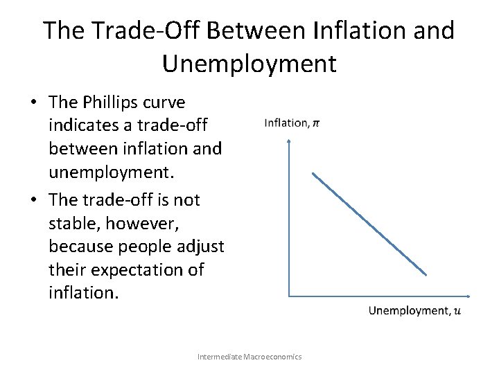
Negative Correlation between Unemployment and Inflation • If the AS curve is upward-sloping and fixed, then shifts of the AD curve predict a negative relationship between unemployment and inflation. – Suppose that the economy is in a recession and that the government conducts fiscal or monetary stimulus, shifting the AD curve to the right. As a result, the output increases, the unemployment rate declines, and the inflation rate picks up. • The Phillips curve describes the trade-off between unemployment and inflation. Intermediate Macroeconomics

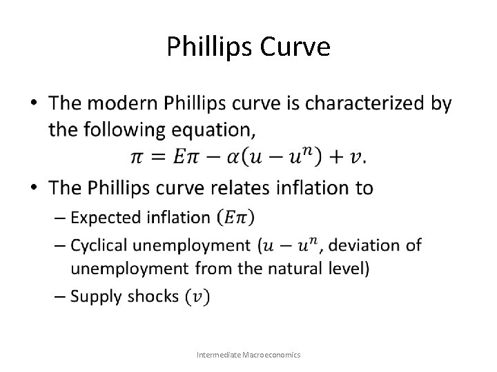
Phillips Curve • Intermediate Macroeconomics

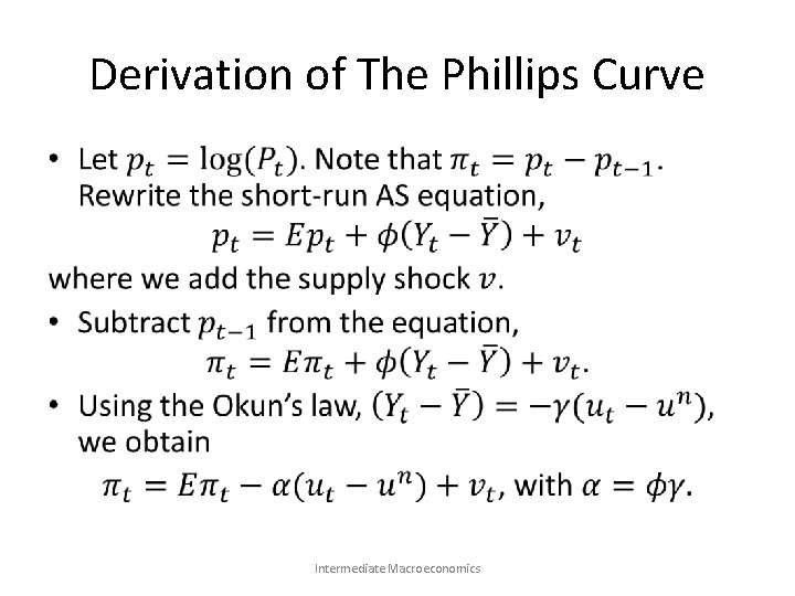
Derivation of The Phillips Curve • Intermediate Macroeconomics

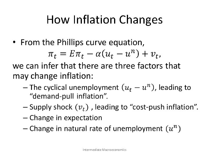
How Inflation Changes • Intermediate Macroeconomics

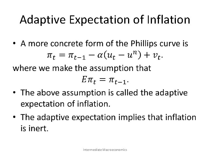
Adaptive Expectation of Inflation • Intermediate Macroeconomics

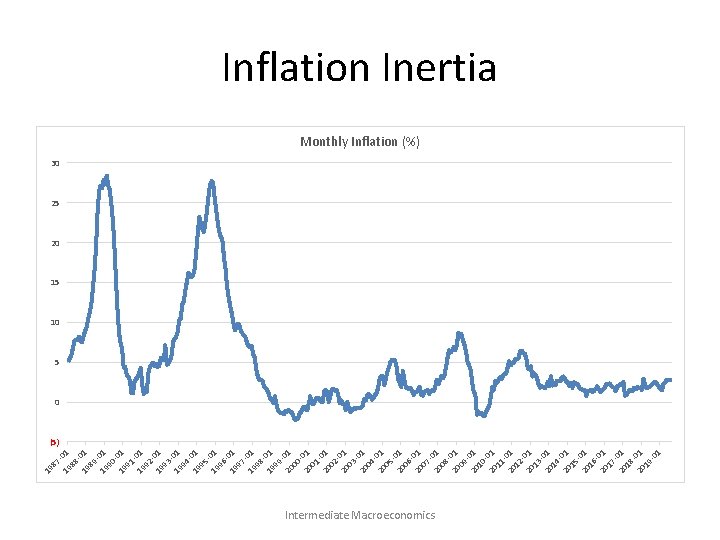
87 19 01 88 19 01 89 19 01 90 19 01 91 19 01 92 19 01 93 19 01 94 19 01 95 19 01 96 19 01 97 19 01 98 19 01 99 20 01 00 20 01 01 20 01 02 20 01 03 20 01 04 20 01 05 20 01 06 20 01 07 20 01 08 20 01 09 20 01 10 20 01 11 20 01 12 20 01 13 20 01 14 20 01 15 20 01 16 20 01 17 20 01 18 20 01 19 -0 1 19 Inflation Inertia Monthly Inflation (%) 30 25 20 15 10 5 0 (5) Intermediate Macroeconomics

The Trade-Off Between Inflation and Unemployment • The Phillips curve indicates a trade-off between inflation and unemployment. • The trade-off is not stable, however, because people adjust their expectation of inflation. Intermediate Macroeconomics

“Sacrifice Ratio” • The trade-off between inflation and output (employment) can be summarized by the “sacrifice ratio”, which is defined by the percentage of a year’s real GDP growth that must be forgone to reduce inflation by 1 percentage point. • In the U. S. , a typical estimate of the sacrifice ratio is about 5: for every percentage point that inflation is to fall, 5 percent of one year’s GDP must be sacrificed. • If the policy of monetary tightening is highly credible, the sacrifice ratio can be much smaller. Intermediate Macroeconomics

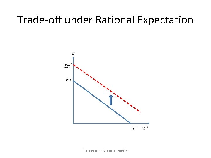
Rational Expectation • Rational expectation is a hypothesis that people form their expectations using all relevant information, and their expectations are correct in average. • Under the rational expectation, there may not be a trade-off between inflation and unemployment. – Bad: it would be futile to combat unemployment with inflation. – Good: it may be painless to combat inflation. In other words, inflation may be brought down without causing any increase in unemployment. • It is important that policies are credible. Intermediate Macroeconomics

Trade-off under Rational Expectation Intermediate Macroeconomics

Natural Rate of Unemployment • It is a hypothesis that there exists a natural rate of unemployment, which is called “natural-rate hypothesis”. • An alternative hypothesis is “hysteresis”, which states that the natural rate of unemployment may be timevarying and the level of unemployment rate depends not only the current state of economy, but also the historical path. – A recession may permanently change an unemployed worker. – A recession may change the balance of “insiders” and “outsiders” in the labor force. Intermediate Macroeconomics

Content • Overview • The IS-LM Models • The AD-AS Model – Aggregate Demand – Aggregate Supply – Phillips Curve – Dynamic AD-AS Model • Keynes Theory • Concluding Remarks Intermediate Macroeconomics

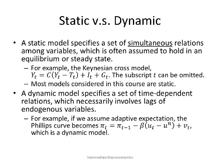
Static v. s. Dynamic • Intermediate Macroeconomics

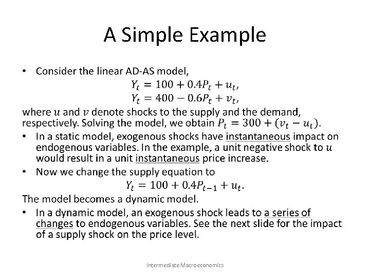
A Simple Example • Intermediate Macroeconomics

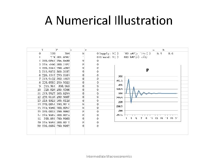
A Numerical Illustration Intermediate Macroeconomics

A More Useful Dynamic AD-AS Model • Model specifications – The IS equation – The “Phillips-curve” equation – A monetary policy rule • Solving the model • Applications Intermediate Macroeconomics

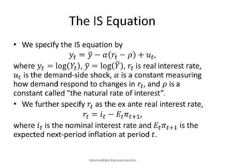
The IS Equation • Intermediate Macroeconomics

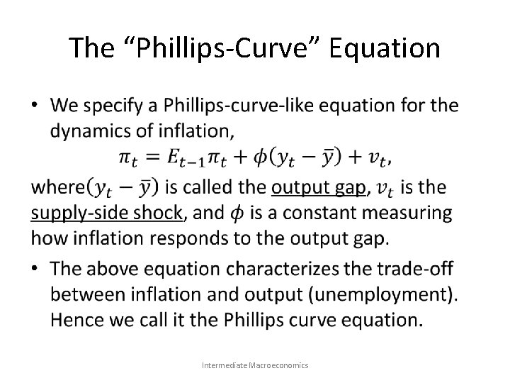
The “Phillips-Curve” Equation • Intermediate Macroeconomics

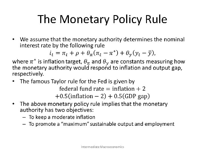
The Monetary Policy Rule • Intermediate Macroeconomics

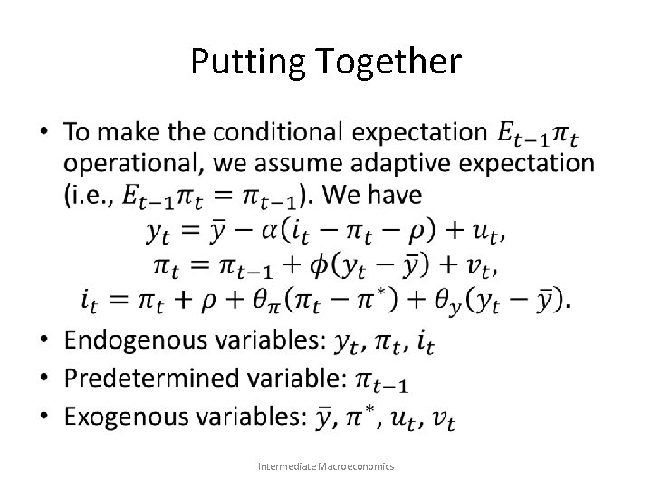
Putting Together • Intermediate Macroeconomics

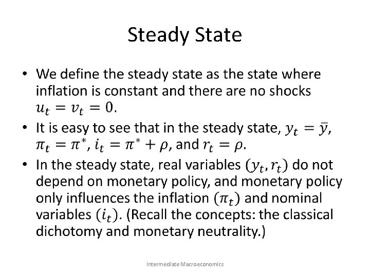
Steady State • Intermediate Macroeconomics

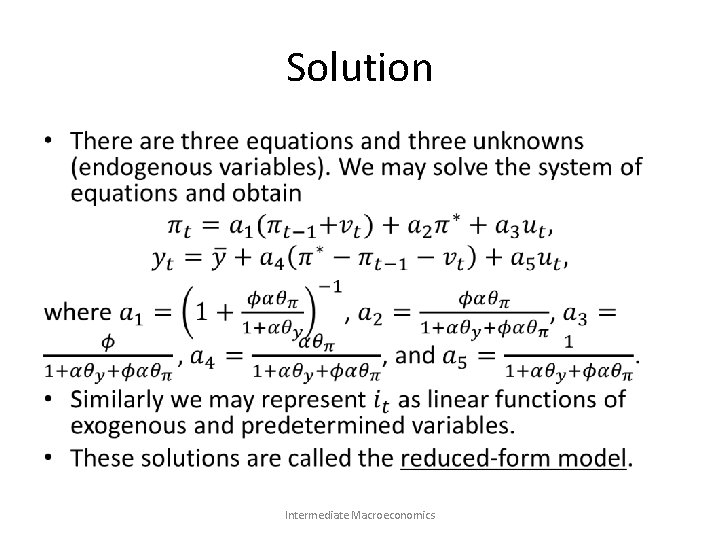
Solution • Intermediate Macroeconomics

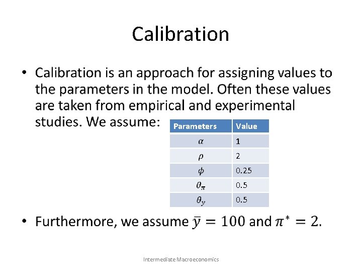
Calibration • Parameters Value 1 2 0. 25 0. 5 Intermediate Macroeconomics

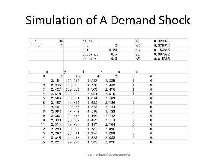
Simulation of A Demand Shock Intermediate Macroeconomics

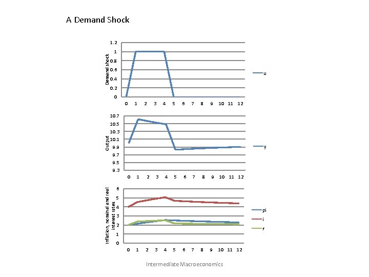
A Demand Shock Demand shock 1. 2 1 0. 8 0. 6 u 0. 4 0. 2 0 0 1 2 3 4 5 6 7 8 9 10 11 12 10. 7 10. 5 Output 10. 3 10. 1 y 9. 9 9. 7 9. 5 9. 3 Inflation, nominal and real interest rates 0 1 2 3 4 5 6 7 8 9 10 11 12 6 5 4 pi 3 i 2 r 1 0 0 1 2 3 4 5 6 7 8 9 10 11 12 Intermediate Macroeconomics

The Economy After A Demand Shock • Intermediate Macroeconomics

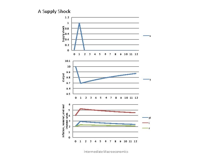
A Supply Shock 1. 2 Supply shock 1 0. 8 0. 6 v 0. 4 0. 2 0 0 1 2 3 4 5 6 7 8 9 10 11 12 10. 1 Output 10 9. 9 9. 8 y 9. 7 9. 6 9. 5 Inflation, nominal, and real interest rates 0 1 2 3 4 5 6 7 8 9 10 11 12 6 5 4 pi 3 i 2 r 1 0 0 1 2 3 4 5 6 7 8 9 10 11 12 Intermediate Macroeconomics

The Economy After A Supply Shock: Stagflation • The supply shock causes the output to decline, the inflation to rise. • Although the supply shock lasts only one period, the inertia of expected inflation keeps the supply curve elevated, leading to prolonged periods of stagnation. • The central bank reacts by raising nominal interest rate more rapidly than inflation. Eventually the central bank would succeed in controlling inflation, but at the cost of a deeper recession. Intermediate Macroeconomics

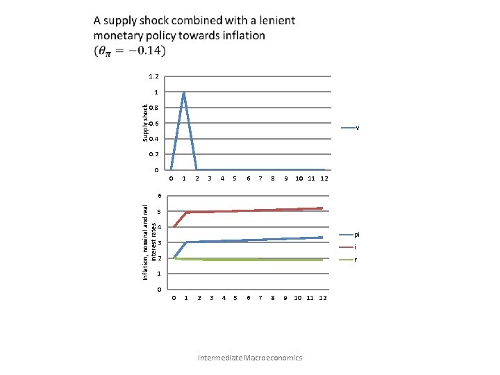
1. 2 Supply shock 1 0. 8 0. 6 v 0. 4 0. 2 0 0 1 2 3 4 5 6 7 8 9 10 11 12 Inflation, nominal and real interest rates 6 5 4 pi 3 i 2 r 1 0 0 1 2 3 4 5 6 7 8 9 10 11 12 Intermediate Macroeconomics

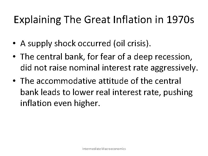
Explaining The Great Inflation in 1970 s • A supply shock occurred (oil crisis). • The central bank, for fear of a deep recession, did not raise nominal interest rate aggressively. • The accommodative attitude of the central bank leads to lower real interest rate, pushing inflation even higher. Intermediate Macroeconomics

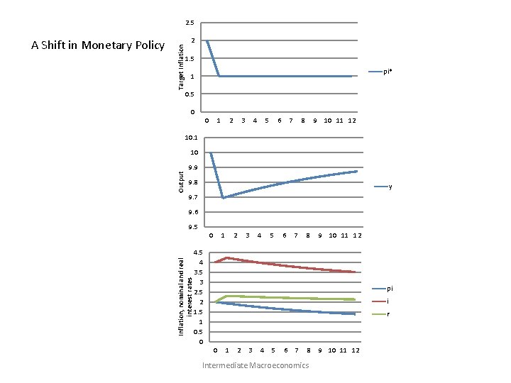
2 1. 5 pi* 1 0. 5 0 0 1 2 3 4 5 6 7 8 9 10 11 12 10. 1 10 Output 9. 9 9. 8 y 9. 7 9. 6 9. 5 0 Inflation, nominal and real interest rates A Shift in Monetary Policy Target Inflation 2. 5 1 2 3 4 5 6 7 8 9 10 11 12 4. 5 4 3. 5 3 2. 5 2 1. 5 1 0. 5 0 pi i r 0 1 2 3 4 5 6 7 8 Intermediate Macroeconomics 9 10 11 12

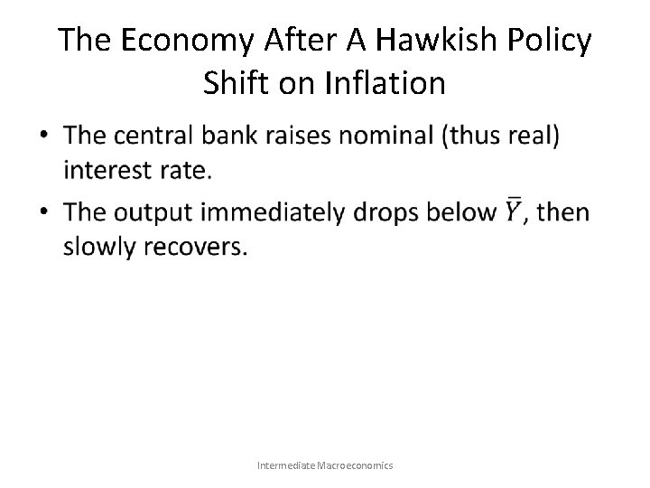
The Economy After A Hawkish Policy Shift on Inflation • Intermediate Macroeconomics

Content • • Overview The IS-LM Models The AD-AS Model Keynes Theory – Theory of Employment – Theory of Investment • Concluding Remarks Intermediate Macroeconomics

The need to study Keynes’ theory • The IS-LM and AD-AS models are interpretations of Keynes’ theory by the mainstream Keynesian or New Keynesian economists. • The mathematical models, however, lose some key insights of Keynes. – The importance of investment – The importance of financial markets Intermediate Macroeconomics

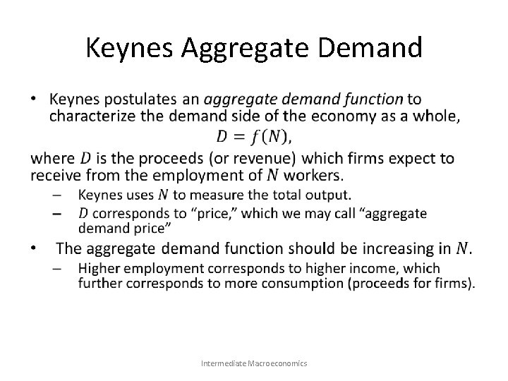
Keynes Aggregate Demand • Intermediate Macroeconomics

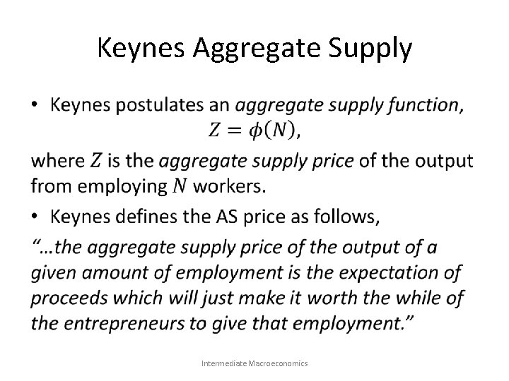
Keynes Aggregate Supply • Intermediate Macroeconomics

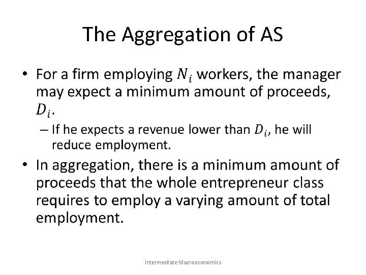
The Aggregation of AS • Intermediate Macroeconomics

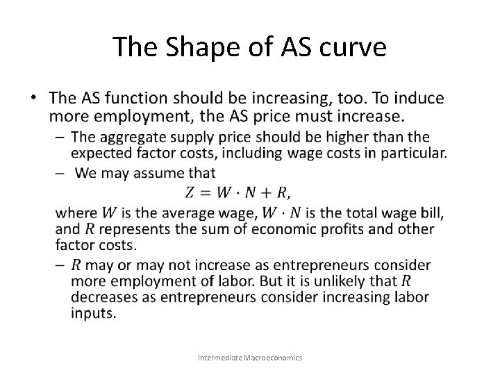
The Shape of AS curve • Intermediate Macroeconomics

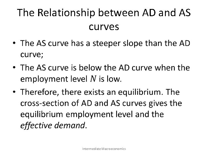
The Relationship between AD and AS curves • Intermediate Macroeconomics

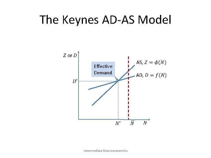
The Keynes AD-AS Model Effective Demand Intermediate Macroeconomics

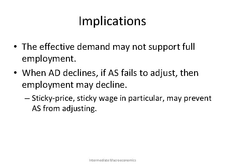
Implications • The effective demand may not support full employment. • When AD declines, if AS fails to adjust, then employment may decline. – Sticky-price, sticky wage in particular, may prevent AS from adjusting. Intermediate Macroeconomics

Content • • Overview The IS-LM Models The AD-AS Model Keynes Theory – Theory of Employment – Theory of Investment • Concluding Remarks Intermediate Macroeconomics

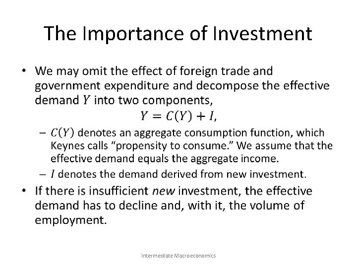
The Importance of Investment • Intermediate Macroeconomics

Paradox of Poverty in the Midst of Plenty • Since the marginal propensity to consume is less than one and it generally declines as income increases, wealthy societies have wider gaps between the aggregate income and the consumption expenditure. • Investment means not only the possibility of future growth but also the necessity of maintaining the current living standards. • Once there is a decline of investment, unemployment will follow. Intermediate Macroeconomics

The Determinants of Investment • Prospective yield: future cash flows from an investment or capital asset. • Supply price, or replacement cost: the asset price that would just induce the production of an additional unit of such assets. • Interest rate Intermediate Macroeconomics

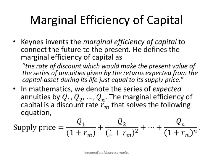
Marginal Efficiency of Capital • Intermediate Macroeconomics

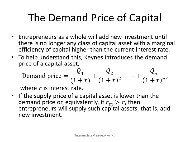
The Demand Price of Capital • Intermediate Macroeconomics

Source of Instability • The supply price of capital is relatively stable. • But the expectation, especially the long-term expectation, of prospective yields can be volatile. • Keyes regards the fluctuation in the marginal efficiency of capital as the cause of business cycles. – The optimistic evaluation of the marginal efficiency of capital leads to over-investment in the later phase of economic expansion. – Sooner or later, the game has to stop since the feverish accumulation of capital would depress the marginal efficiency of capital. When this happens, optimism gives way to pessimism. Intermediate Macroeconomics

When Does a Recession End? • The recession continues as long as the marginal efficiency of capital is lower than the interest rate. The dismal state of the economy may change for the better when: – the monetary authority slashes the interest rate to below the marginal efficiency of capital; – the expectation of future yield improves as business confidence restores; – the supply price of capital declines by an amount enough for the marginal efficiency of capital to exceed the rate of interest. Intermediate Macroeconomics

The Role of the Stock Market • For potential entrepreneurs, stocks are alternatives to investment in real assets. – When stock market valuation is low, there is little incentive for entrepreneurs to make new investments since they can purchase capital assets in the stock market. • The stock market provides for entrepreneurs and investors with a conventional valuation on almost every type of capital asset. – The conventional valuation is imperfect but indispensable. • Uncertainty makes it difficult to form expectations about prospective yields. Intermediate Macroeconomics

The Weaknesses of the Stock Market 1. The stock market’s overall ability to value assets is dubious. 2. Short-term fluctuations in profits tend to have excessive influence on the market. 3. The conventional valuation of the stock market results from the mass psychology of a large number of ignorant individuals, which may suddenly change due to factors unrelated to the prospective yield. Intermediate Macroeconomics

The Weaknesses of the Stock Market 4. Even professional investors and speculators are concerned not with making superior forecasts of future yields, but with foreseeing changes in the conventional valuation a little ahead of the others. – Challenges for value investors a) Human nature desires quick results. b) The value investors must have greater resources for safety and should avoid leverage. c) When a committee is in charge of evaluating investment performance, the value investor will face the most criticism. Intermediate Macroeconomics

Summary of Keynes’ View • The conventional valuation offered by the stock market has deep flaws. • The violent fluctuations in the mass psychology of investors and speculators drive the fluctuations in the conventional valuation of prospective yields, which further drives the fluctuations in new investment, which further drives the business cycles. • Keynes: When the capital development of a country becomes a by-product of the activities of a casino, the job is likely to be ill-done. Intermediate Macroeconomics

Content • • • Overview The IS-LM Models The AD-AS Model Keynes Theory Concluding Remarks Intermediate Macroeconomics

Concluding Remarks on Business Cycles • The full-employment equilibrium is as “transitory” as the under-employment equilibria. • Full of inner dynamism, our economy cannot stay quietly anywhere. As soon as it recovers from a recession and reaches the fullemployment state, it will move on to overheat. • The inner dynamism manifests itself most evidently in finance. Intermediate Macroeconomics

Minsky’s Financial Instability Hypothesis • Minsky: A fundamental characteristic of our economy is that the financial system swings between robustness and fragility and these swings are an integral part of the process that generates business cycles. Intermediate Macroeconomics

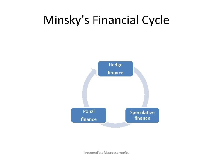
Minsky’s Financial Cycle Hedge finance Ponzi finance Intermediate Macroeconomics Speculative finance

Concluding Remarks on Business Cycles • The financial cycle does not simply repeat in the same style. Every cycle is different because financial markets are structurally changing over time. – The government reaction to busts (and booms): regulation and deregulation. – The market reactions: financial innovations, shadow banks. • Mark Twain: The history of economic fluctuations doesn't repeat itself, but it often rhymes. Intermediate Macroeconomics