Factor Analysis QianLi Xue Biostatistics Program Harvard Catalyst

Factor Analysis Qian-Li Xue Biostatistics Program Harvard Catalyst | The Harvard Clinical & Translational Science Center Short course, October 27, 2016 1

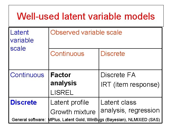
Well-used latent variable models Latent variable scale Observed variable scale Continuous Factor analysis LISREL Discrete Latent profile Growth mixture Discrete FA IRT (item response) Latent class analysis, regression General software: MPlus, Latent Gold, Win. Bugs (Bayesian), NLMIXED (SAS)

Objectives § What is factor analysis? § What do we need factor analysis for? § What are the modeling assumptions? § How to specify, fit, and interpret factor models? § What is the difference between exploratory and confirmatory factor analysis? § What is and how to assess model identifiability? 3

What is factor analysis § Factor analysis is a theory driven statistical data reduction technique used to explain covariance among observed random variables in terms of fewer unobserved random variables named factors 4

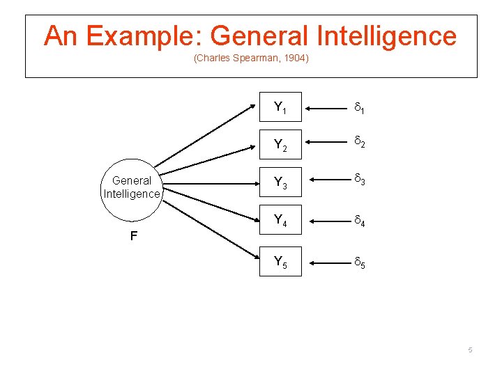
An Example: General Intelligence (Charles Spearman, 1904) General Intelligence Y 1 1 Y 2 2 Y 3 3 Y 4 4 Y 5 5 F 5

Why Factor Analysis? 1. Testing of theory § Explain covariation among multiple observed variables by § Mapping variables to latent constructs (called “factors”) 2. Understanding the structure underlying a set of measures § Gain insight to dimensions § Construct validation (e. g. , convergent validity) 3. Scale development § Exploit redundancy to improve scale’s validity and reliability 6

Part I. Exploratory Factor Analysis (EFA) 7

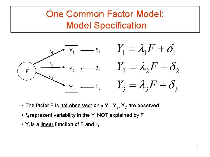
One Common Factor Model: Model Specification 1 2 F Y 1 1 Y 2 2 Y 3 3 3 § The factor F is not observed; only Y 1, Y 2, Y 3 are observed § i represent variability in the Yi NOT explained by F § Yi is a linear function of F and i 8

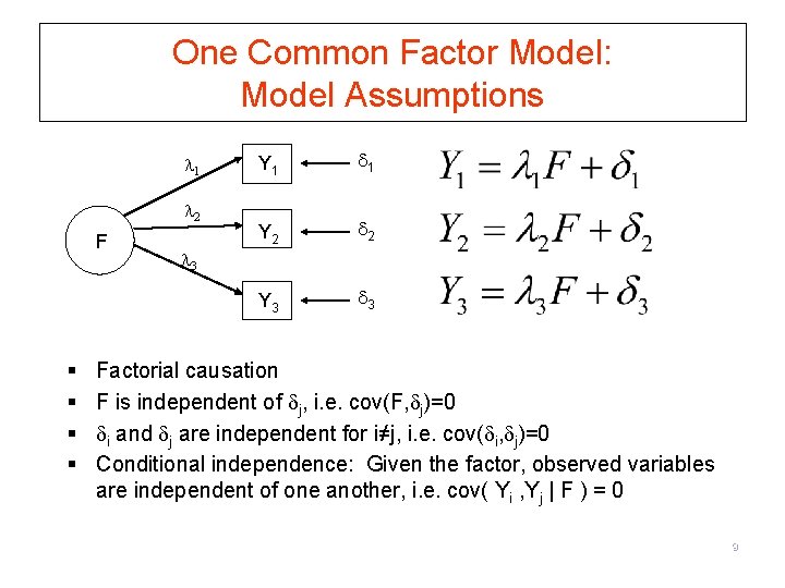
One Common Factor Model: Model Assumptions 1 2 F § § Y 1 1 Y 2 2 Y 3 3 3 Factorial causation F is independent of j, i. e. cov(F, j)=0 i and j are independent for i≠j, i. e. cov( i, j)=0 Conditional independence: Given the factor, observed variables are independent of one another, i. e. cov( Yi , Yj | F ) = 0 9

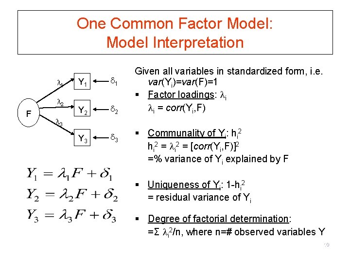
One Common Factor Model: Model Interpretation 1 2 F Y 1 1 Y 2 2 Y 3 3 Given all variables in standardized form, i. e. var(Yi)=var(F)=1 § Factor loadings: i i = corr(Yi, F) 3 § Communality of Yi: hi 2 = [corr(Yi, F)]2 =% variance of Yi explained by F § Uniqueness of Yi: 1 -hi 2 = residual variance of Yi § Degree of factorial determination: =Σ i 2/n, where n=# observed variables Y 10

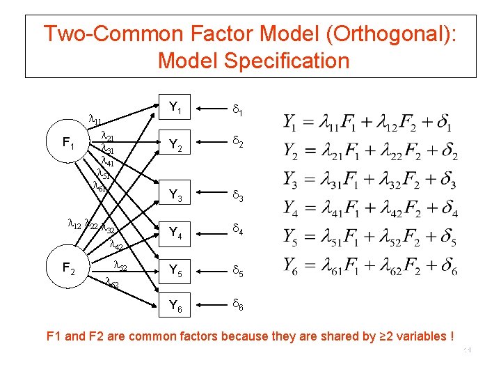
Two-Common Factor Model (Orthogonal): Model Specification F 1 11 21 31 41 51 61 12 22 32 42 F 2 52 62 Y 1 1 Y 2 2 Y 3 3 Y 4 4 Y 5 5 Y 6 6 F 1 and F 2 are common factors because they are shared by ≥ 2 variables ! 11

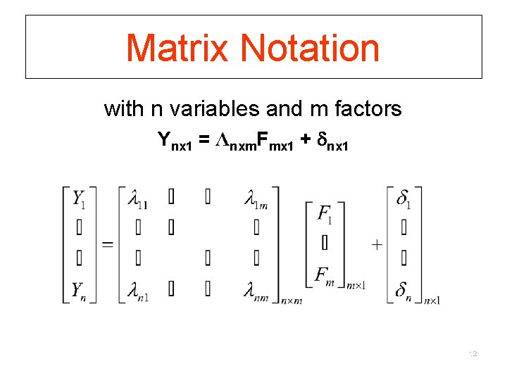
Matrix Notation with n variables and m factors Ynx 1 = Λnxm. Fmx 1 + nx 1 12

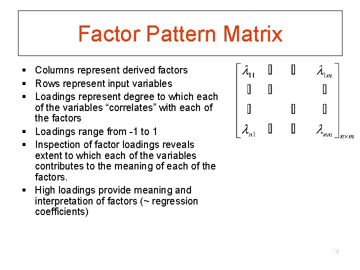
Factor Pattern Matrix § Columns represent derived factors § Rows represent input variables § Loadings represent degree to which each of the variables “correlates” with each of the factors § Loadings range from -1 to 1 § Inspection of factor loadings reveals extent to which each of the variables contributes to the meaning of each of the factors. § High loadings provide meaning and interpretation of factors (~ regression coefficients) 13

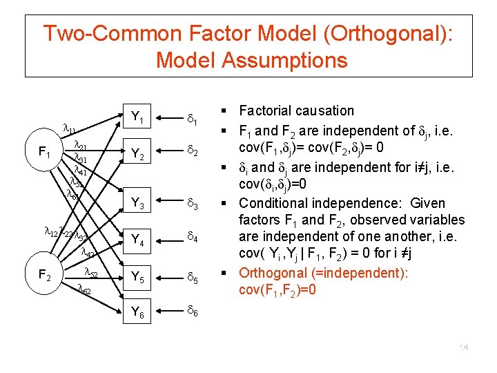
Two-Common Factor Model (Orthogonal): Model Assumptions F 1 11 21 31 41 51 61 12 22 32 42 F 2 52 62 Y 1 1 Y 2 2 Y 3 3 Y 4 4 Y 5 5 Y 6 6 § Factorial causation § F 1 and F 2 are independent of j, i. e. cov(F 1, j)= cov(F 2, j)= 0 § i and j are independent for i≠j, i. e. cov( i, j)=0 § Conditional independence: Given factors F 1 and F 2, observed variables are independent of one another, i. e. cov( Yi , Yj | F 1, F 2) = 0 for i ≠j § Orthogonal (=independent): cov(F 1, F 2)=0 14

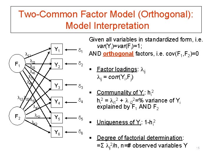
Two-Common Factor Model (Orthogonal): Model Interpretation F 1 11 21 31 41 51 61 12 22 32 42 F 2 52 62 Y 1 1 Y 2 2 Y 3 3 Y 4 4 Y 5 5 Y 6 6 Given all variables in standardized form, i. e. var(Yi)=var(Fi)=1; AND orthogonal factors, i. e. cov(F 1, F 2)=0 § Factor loadings: ij ij = corr(Yi, Fj) § Communality of Yi: hi 2 = i 12 + i 22=% variance of Yi explained by F 1 AND F 2 § Uniqueness of Yi: 1 -hi 2 § Degree of factorial determination: =Σ ij 2/n, n=# observed variables Y 15

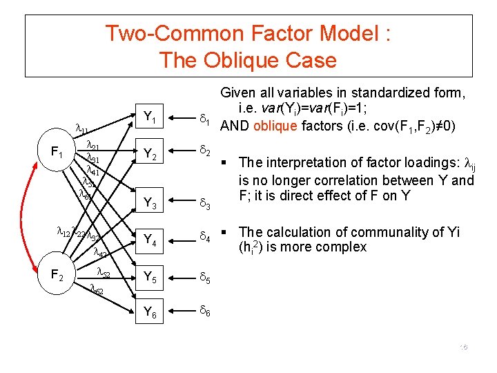
Two-Common Factor Model : The Oblique Case F 1 11 21 31 41 51 61 12 22 32 42 F 2 52 62 Given all variables in standardized form, i. e. var(Yi)=var(Fi)=1; AND oblique factors (i. e. cov(F 1, F 2)≠ 0) Y 1 1 Y 2 2 Y 3 3 Y 4 4 § The calculation of communality of Yi Y 5 5 Y 6 6 § The interpretation of factor loadings: ij is no longer correlation between Y and F; it is direct effect of F on Y (hi 2) is more complex 16

Extracting initial factors § § Least-squares method (e. g. principal axis factoring with iterated communalities) Maximum likelihood method 17

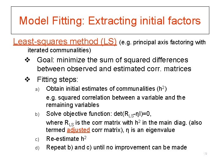
Model Fitting: Extracting initial factors Least-squares method (LS) (e. g. principal axis factoring with iterated communalities) v Goal: minimize the sum of squared differences between observed and estimated corr. matrices v Fitting steps: a) b) c) d) Obtain initial estimates of communalities (h 2) e. g. squared correlation between a variable and the remaining variables Solve objective function: det(RLS-ηI)=0, where RLS is the corr matrix with h 2 in the main diag. (also termed adjusted corr matrix), η is an eigenvalue Re-estimate h 2 Repeat b) and c) until no improvement can be made 18

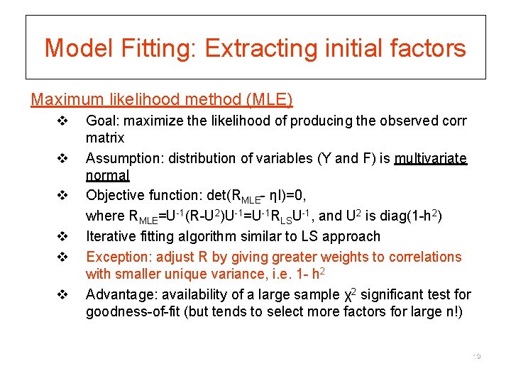
Model Fitting: Extracting initial factors Maximum likelihood method (MLE) v v v Goal: maximize the likelihood of producing the observed corr matrix Assumption: distribution of variables (Y and F) is multivariate normal Objective function: det(RMLE- ηI)=0, where RMLE=U-1(R-U 2)U-1=U-1 RLSU-1, and U 2 is diag(1 -h 2) Iterative fitting algorithm similar to LS approach Exception: adjust R by giving greater weights to correlations with smaller unique variance, i. e. 1 - h 2 Advantage: availability of a large sample χ2 significant test for goodness-of-fit (but tends to select more factors for large n!) 19

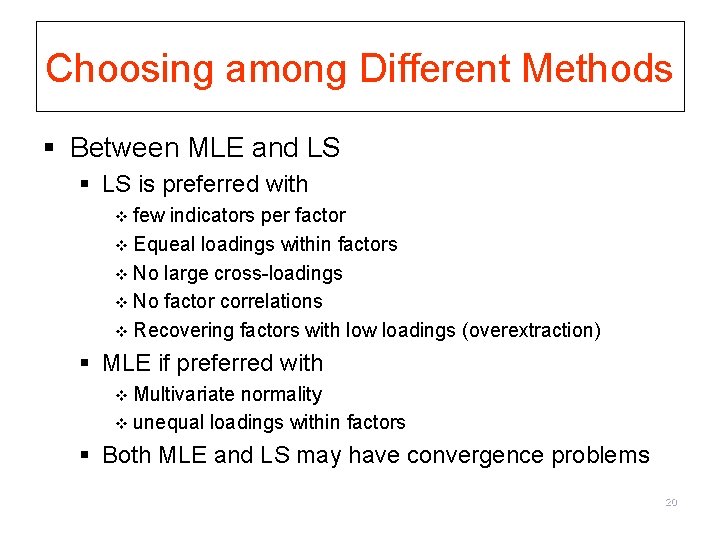
Choosing among Different Methods § Between MLE and LS § LS is preferred with v few indicators per factor v Equeal loadings within factors v No large cross-loadings v No factor correlations v Recovering factors with low loadings (overextraction) § MLE if preferred with v Multivariate normality v unequal loadings within factors § Both MLE and LS may have convergence problems 20

Factor Rotation § Goal is simple structure § Make factors more easily interpretable § While keeping the number of factors and communalities of Ys fixed!!! § Rotation does NOT improve fit! 21

Factor Rotation To do this we “rotate” factors: § redefine factors such that ‘loadings’ (or pattern matrix coefficients) on various factors tend to be very high (-1 or 1) or very low (0) § intuitively, it makes sharper distinctions in the meanings of the factors 22

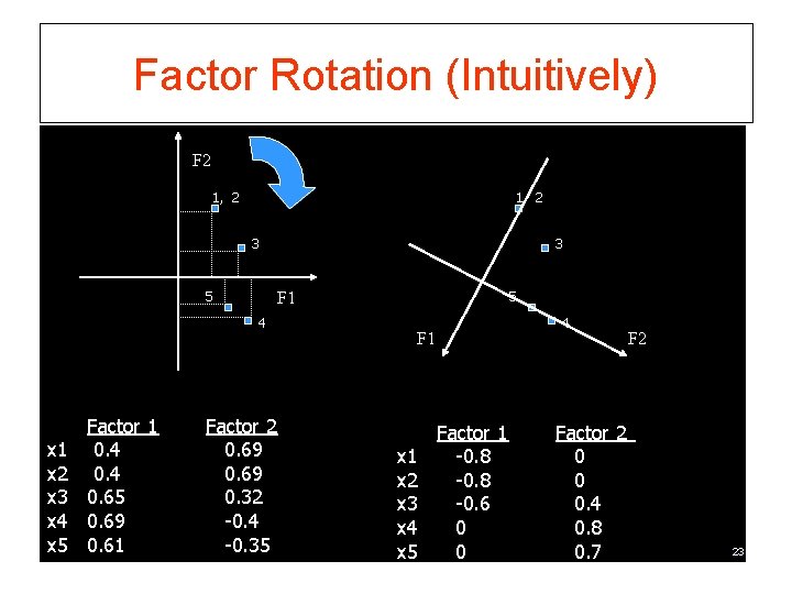
Factor Rotation (Intuitively) F 2 1, 2 3 5 3 4 x 1 x 2 x 3 x 4 x 5 Factor 1 0. 4 0. 65 0. 69 0. 61 5 F 1 Factor 2 0. 69 0. 32 -0. 4 -0. 35 4 F 1 x 2 x 3 x 4 x 5 Factor 1 -0. 8 -0. 6 0 0 Factor 2 0 0 0. 4 0. 8 0. 7 F 2 23

Factor Rotation § Uses “ambiguity” or non-uniqueness of solution to make interpretation more simple § Where does ambiguity come in? § Unrotated solution is based on the idea that each factor tries to maximize variance explained, conditional on previous factors § What if we take that away? § Then, there is not one “best” solution 24

Factor Rotation: Orthogonal vs. Oblique Rotation § Orthogonal: Factors are independent § varimax: maximize variance of squared loadings across variables (sum over factors) v Goal: the simplicity of interpretation of factors § quartimax: maximize variance of squared loadings across factors (sum over variables) v Goal: the simplicity of interpretation of variables § Intuition: from previous picture, there is a right angle between axes § Note: “Uniquenesses” remain the same! 25

Factor Rotation: Orthogonal vs. Oblique Rotation § Oblique: Factors are NOT independent. Change in “angle. ” § oblimin: minimize covariance of squared loadings between factors. § promax: simplify orthogonal rotation by making small loadings even closer to zero. § Target matrix: choose “simple structure” a priori. § Intuition: from previous picture, angle between axes is not necessarily a right angle. § Note: “Uniquenesses” remain the same! 26

Pattern versus Structure Matrix § In oblique rotation, one typically presents both a pattern matrix and a structure matrix § Also need to report correlation between the factors § The pattern matrix presents the usual factor loadings § The structure matrix presents correlations between the variables and the factors § For orthogonal factors, pattern matrix=structure matrix § The pattern matrix is used to interpret the factors 27

Factor Rotation: Which to use? § Choice is generally not critical § Interpretation with orthogonal (varimax) is “simple” because factors are independent: “Loadings” are correlations. § Configuration may appear more simple in oblique (promax), but correlation of factors can be difficult to reconcile. § Theory? Are the conceptual meanings of the factors associated? 28

Factor Rotation: Unique Solution? § The factor analysis solution is NOT unique! § More than one solution will yield the same “result. ” 29

Derivation of Factor Scores § Each object (e. g. each person) gets a factor score for each factor: § The factors themselves are variables § “Object’s” score is weighted combination of scores on input variables § § These weights are NOT the factor loadings! Different approaches exist for estimating (e. g. regression method) Factor scores are not unique Using factors scores instead of factor indicators can reduce measurement error, but does NOT remove it. § Therefore, using factor scores as predictors in conventional regressions leads to inconsistent coefficient estimators! 30

Factor Analysis with Categorical Observed Variables § Factor analysis hinges on the correlation matrix § As long as you can get an interpretable correlation matrix, you can perform factor analysis § Binary/ordinal items? § Pearson corrlation: Expect attenuation! § Tetrachoric correlation (binary) § Polychoric correlation (ordinal) To obtain polychoric correlation in STATA: polychoric var 1 var 2 var 3 var 4 var 5 … To run princial component analysis: pcamat r(R), n(328) To run factor analysis: factormat r(R), fa(2) ipf n(328) 31

Criticisms of Factor Analysis § Labels of factors can be arbitrary or lack scientific basis § Derived factors often very obvious § defense: but we get a quantification § “Garbage in, garbage out” § really a criticism of input variables § factor analysis reorganizes input matrix § Correlation matrix is often poor measure of association of input variables. 32

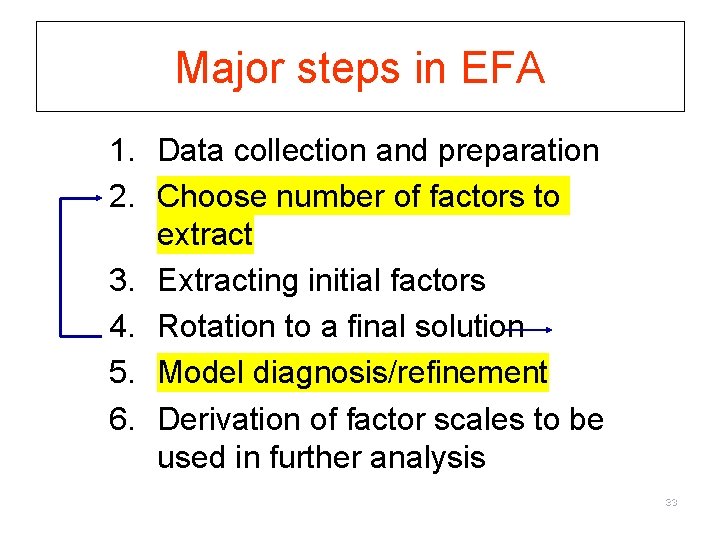
Major steps in EFA 1. Data collection and preparation 2. Choose number of factors to extract 3. Extracting initial factors 4. Rotation to a final solution 5. Model diagnosis/refinement 6. Derivation of factor scales to be used in further analysis 33

Part II. Confirmatory Factor Analysis (CFA) 34

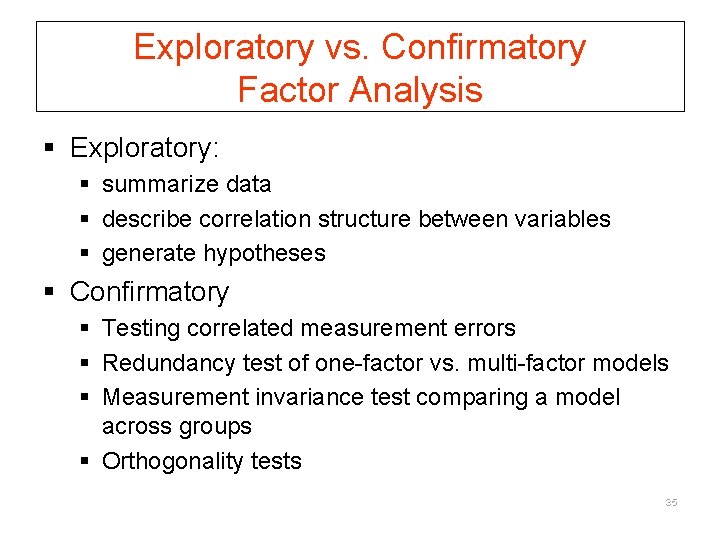
Exploratory vs. Confirmatory Factor Analysis § Exploratory: § summarize data § describe correlation structure between variables § generate hypotheses § Confirmatory § Testing correlated measurement errors § Redundancy test of one-factor vs. multi-factor models § Measurement invariance test comparing a model across groups § Orthogonality tests 35

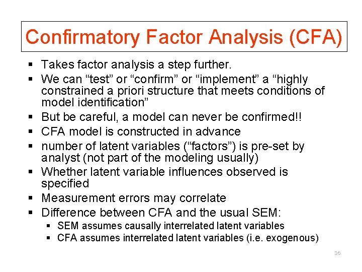
Confirmatory Factor Analysis (CFA) § Takes factor analysis a step further. § We can “test” or “confirm” or “implement” a “highly constrained a priori structure that meets conditions of model identification” § But be careful, a model can never be confirmed!! § CFA model is constructed in advance § number of latent variables (“factors”) is pre-set by analyst (not part of the modeling usually) § Whether latent variable influences observed is specified § Measurement errors may correlate § Difference between CFA and the usual SEM: § SEM assumes causally interrelated latent variables § CFA assumes interrelated latent variables (i. e. exogenous) 36

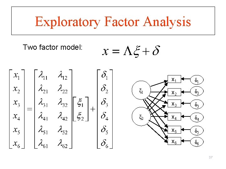
Exploratory Factor Analysis Two factor model: ξ 1 ξ 2 x 1 δ 1 x 2 δ 2 x 3 δ 3 x 4 δ 4 x 5 δ 5 x 6 δ 6 37

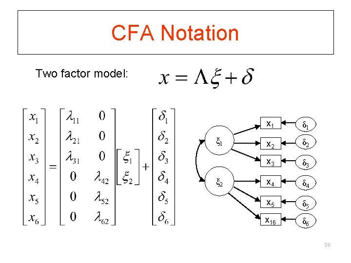
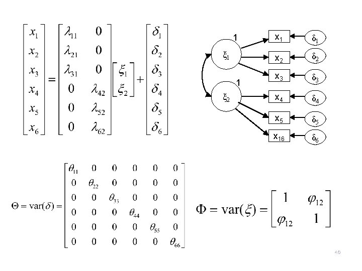
CFA Notation Two factor model: ξ 1 ξ 2 x 1 δ 1 x 2 δ 2 x 3 δ 3 x 4 δ 4 x 5 δ 5 x 16 δ 6 38

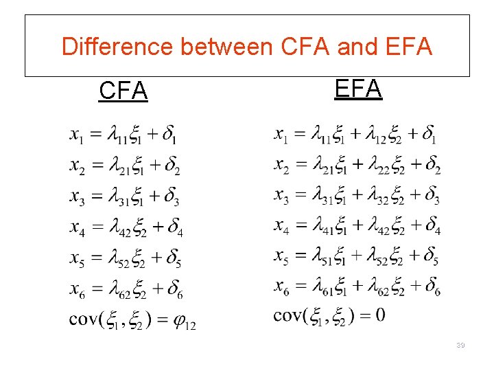
Difference between CFA and EFA CFA EFA 39

Model Constraints § Hallmark of CFA § Purposes for setting constraints: § Test a priori theory § Ensure identifiability § Test reliability of measures 40

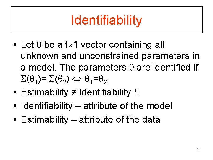
Identifiability § Let be a t 1 vector containing all unknown and unconstrained parameters in a model. The parameters are identified if ( 1)= ( 2) 1= 2 § Estimability ≠ Identifiability !! § Identifiability – attribute of the model § Estimability – attribute of the data 41

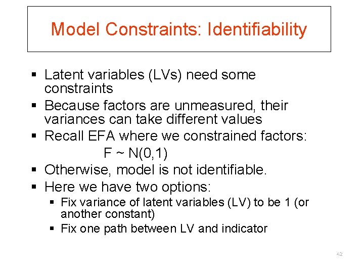
Model Constraints: Identifiability § Latent variables (LVs) need some constraints § Because factors are unmeasured, their variances can take different values § Recall EFA where we constrained factors: F ~ N(0, 1) § Otherwise, model is not identifiable. § Here we have two options: § Fix variance of latent variables (LV) to be 1 (or another constant) § Fix one path between LV and indicator 42

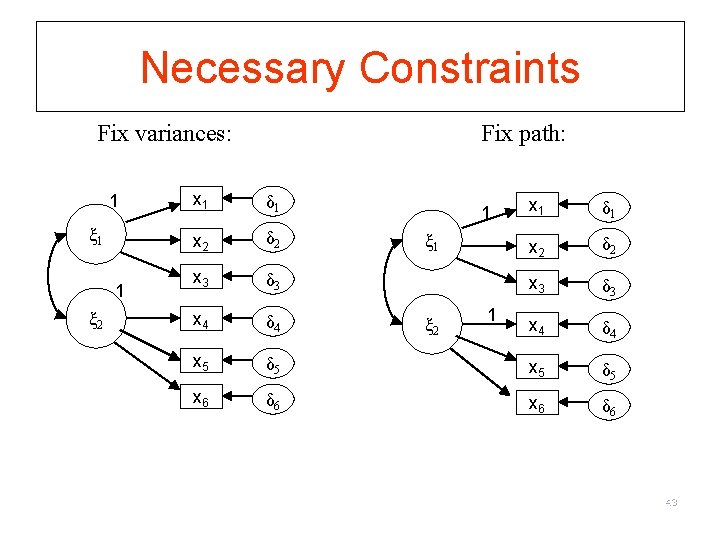
Necessary Constraints Fix variances: 1 ξ 1 1 ξ 2 Fix path: x 1 δ 1 x 2 δ 2 x 3 δ 3 x 4 δ 4 x 5 x 6 x 1 δ 1 x 2 δ 2 x 3 δ 3 x 4 δ 5 x 5 δ 6 x 6 δ 6 1 ξ 2 1 43

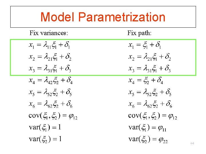
Model Parametrization Fix variances: Fix path: 44

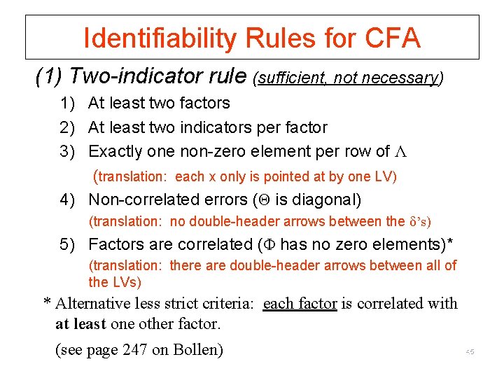
Identifiability Rules for CFA (1) Two-indicator rule (sufficient, not necessary) 1) At least two factors 2) At least two indicators per factor 3) Exactly one non-zero element per row of Λ (translation: each x only is pointed at by one LV) 4) Non-correlated errors (Θ is diagonal) (translation: no double-header arrows between the δ’s) 5) Factors are correlated (Φ has no zero elements)* (translation: there are double-header arrows between all of the LVs) * Alternative less strict criteria: each factor is correlated with at least one other factor. (see page 247 on Bollen) 45

1 ξ 1 1 ξ 2 x 1 δ 1 x 2 δ 2 x 3 δ 3 x 4 δ 4 x 5 δ 5 x 16 δ 6 46

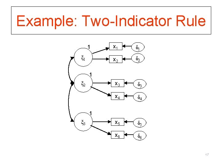
Example: Two-Indicator Rule 1 ξ 1 x 1 δ 1 x 2 δ 2 1 ξ 2 x 3 δ 3 x 4 δ 4 x 5 δ 5 x 6 δ 6 1 ξ 3 47

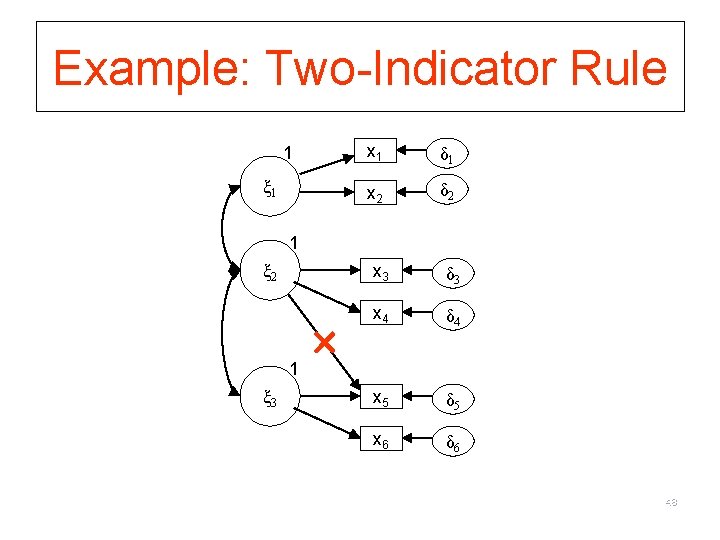
Example: Two-Indicator Rule 1 ξ 1 x 1 δ 1 x 2 δ 2 1 ξ 3 x 3 δ 3 x 4 δ 4 x 5 δ 5 x 6 δ 6 48

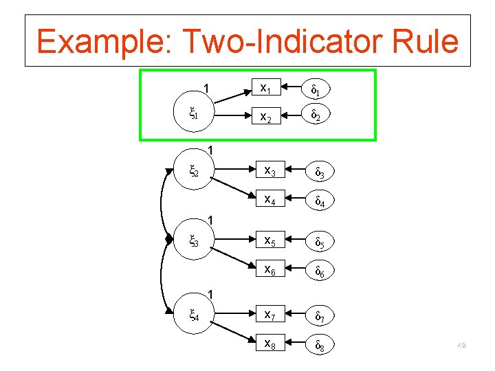
Example: Two-Indicator Rule 1 ξ 1 x 1 δ 1 x 2 δ 2 1 ξ 2 x 3 δ 3 x 4 δ 4 x 5 δ 5 x 6 δ 6 x 7 δ 7 x 8 δ 8 1 ξ 3 1 ξ 4 49

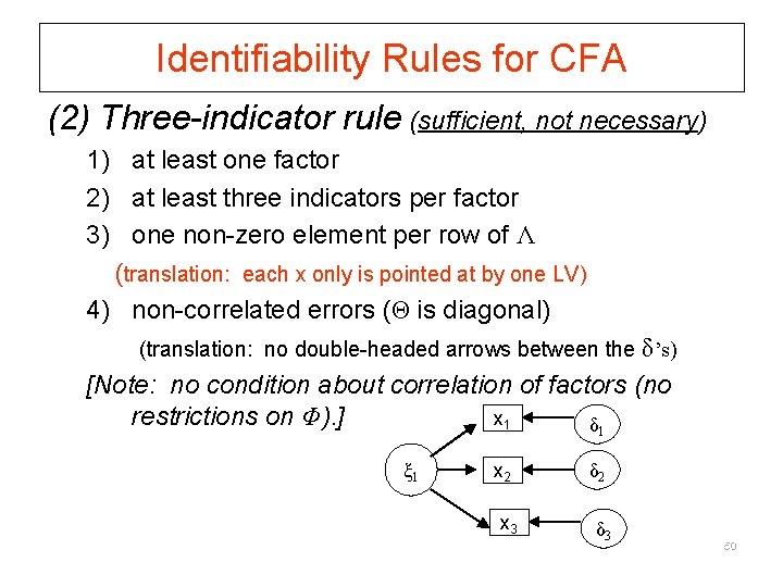
Identifiability Rules for CFA (2) Three-indicator rule (sufficient, not necessary) 1) at least one factor 2) at least three indicators per factor 3) one non-zero element per row of Λ (translation: each x only is pointed at by one LV) 4) non-correlated errors (Θ is diagonal) (translation: no double-headed arrows between the δ’s) [Note: no condition about correlation of factors (no x 1 restrictions on Φ). ] δ 1 ξ 1 x 2 x 3 δ 2 δ 3 50