Multilevel Discretetime Event History Analysis Centre for Multilevel

Multilevel Discrete-time Event History Analysis Centre for Multilevel Modelling Graduate School of Education University of Bristol 13 -14 September 2007 Instructor: Fiona Steele

Course Outline • Discrete-time methods for modelling time to a single event • Multilevel models for recurrent events and unobserved heterogeneity • Modelling transitions between multiple states • Modelling competing risks • Multiprocess models for correlated histories Multilevel Discrete-Time Event History Analysis 2

Discrete-time Methods for Modelling the Time to a Single Event

What is Event History Analysis? Methods for analysis of length of time until the occurrence of some event. The dependent variable is the duration until event occurrence. EHA also known as: • Survival analysis (particularly in biostatistics and when event is not repeatable) • Duration analysis • Hazard modelling Multilevel Discrete-Time Event History Analysis 4

Examples of Applications • Education – time to leaving full-time education (from end of compulsory education); time to exit from teaching profession • Economics – duration of an episode of unemployment or employment • Demography – time to first birth (from when? ); time to first marriage; time to divorce • Psychology – duration to response to some stimulus Multilevel Discrete-Time Event History Analysis 5

Special Features of Event History Data • Durations are always positive and their distribution is often skewed • Censoring – there are usually people who have not yet experienced the event when we observe them • Time-varying covariates – the values of some covariates may change over time Multilevel Discrete-Time Event History Analysis 6

Censoring (1) Multilevel Discrete-Time Event History Analysis 7

Censoring (2) Multilevel Discrete-Time Event History Analysis 8

Right-censoring: Non-informative Assumption Excluding right-censored observations leads to bias and may drastically reduce sample size. In EHA we retain these observations and usually make the assumption that censoring is non-informative, i. e. event times are independent of censoring mechanism (like the ‘missing at random’ assumption). Assume individuals are not selectively withdrawn from the sample because they are more or less likely to experience an event. May be questionable in experimental research, e. g. if more susceptible individuals were selectively withdrawn from a ‘treatment’ group. Multilevel Discrete-Time Event History Analysis 9

Event Times and Censoring Times Multilevel Discrete-Time Event History Analysis 10

The Discrete-time Approach Event times measured in discrete intervals t=1, 2, 3, . . . (e. g. months, years). Can think of event history as a series of independent success/failure trials. In each interval t we observe a binary response indicating whether an event has occurred. Multilevel Discrete-Time Event History Analysis 11

Main Advantages of the Discrete-time Approach • Events times often measured in discrete-time units, particularly when collected retrospectively • Allows proportional hazards assumption to be tested straightforwardly. Straightforward to allow for nonproportional hazards. • Analysis straightforward as we can use models for discrete response data – important for more complex data structures and processes Multilevel Discrete-Time Event History Analysis 12

Disadvantages of the Discrete-time Approach • Data must first be restructured so that for each individual we have a sequence of observations, one for each time interval until event occurrence or censoring. • If observation period is long relative to the width of the time intervals in which durations are measured, the dataset may become very large. Multilevel Discrete-Time Event History Analysis 13

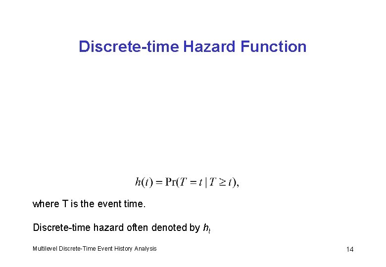
Discrete-time Hazard Function where T is the event time. Discrete-time hazard often denoted by ht Multilevel Discrete-Time Event History Analysis 14

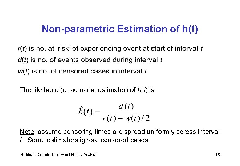
Non-parametric Estimation of h(t) The life table (or actuarial estimator) of h(t) is Note: assume censoring times are spread uniformly across interval t. Some estimators ignore censored cases. Multilevel Discrete-Time Event History Analysis 15

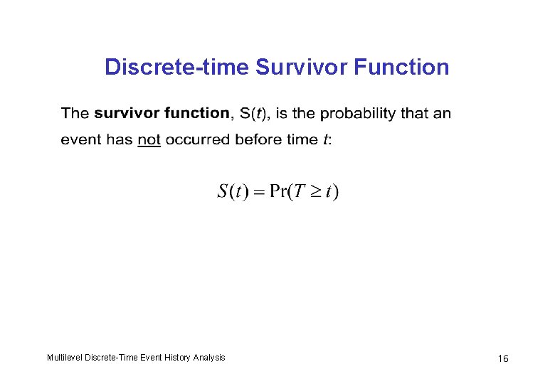
Discrete-time Survivor Function Multilevel Discrete-Time Event History Analysis 16

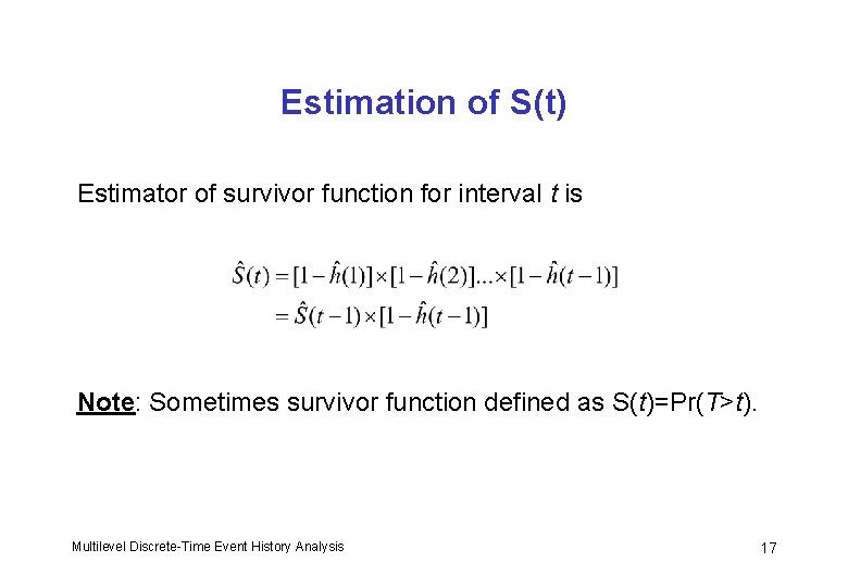
Estimation of S(t) Estimator of survivor function for interval t is Note: Sometimes survivor function defined as S(t)=Pr(T>t). Multilevel Discrete-Time Event History Analysis 17

Restructuring Data for a Discrete-time Analysis: Individual-based File Multilevel Discrete-Time Event History Analysis 18

Restructuring Data for a Discrete-time Analysis: Discrete-time (Person-period) File Multilevel Discrete-Time Event History Analysis 19

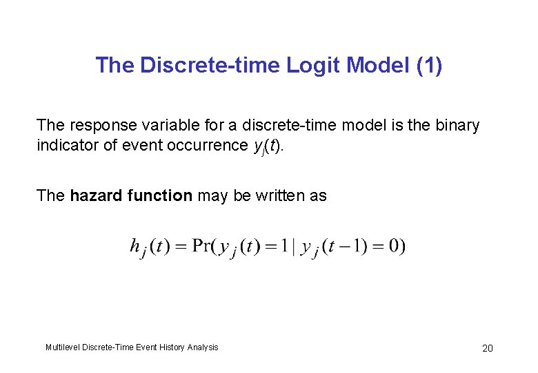
The Discrete-time Logit Model (1) The response variable for a discrete-time model is the binary indicator of event occurrence yj(t). The hazard function may be written as Multilevel Discrete-Time Event History Analysis 20

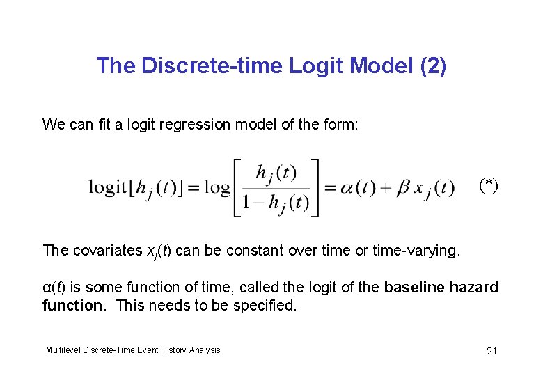
The Discrete-time Logit Model (2) We can fit a logit regression model of the form: (*) The covariates xj(t) can be constant over time or time-varying. α(t) is some function of time, called the logit of the baseline hazard function. This needs to be specified. Multilevel Discrete-Time Event History Analysis 21

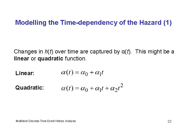
Modelling the Time-dependency of the Hazard (1) Changes in h(t) over time are captured by α(t). This might be a linear or quadratic function. Linear: Quadratic: Multilevel Discrete-Time Event History Analysis 22

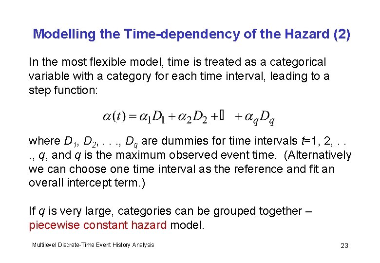
Modelling the Time-dependency of the Hazard (2) In the most flexible model, time is treated as a categorical variable with a category for each time interval, leading to a step function: where D 1, D 2, . . . , Dq are dummies for time intervals t=1, 2, . . . , q, and q is the maximum observed event time. (Alternatively we can choose one time interval as the reference and fit an overall intercept term. ) If q is very large, categories can be grouped together – piecewise constant hazard model. Multilevel Discrete-Time Event History Analysis 23

The Proportional Hazards Assumption Model (*) assumes that the effects of covariates x(t) are constant over time. This is known as the proportional hazards assumption. (Strictly it is the odds that are assumed proportional as we are fitting a logit model. ) We can relax this assumption by introducing interactions between x(t) and α(t). Multilevel Discrete-Time Event History Analysis 24

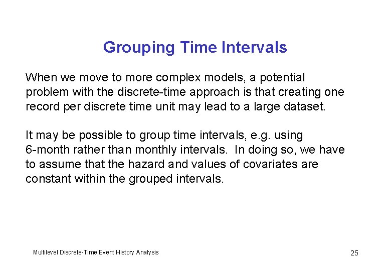
Grouping Time Intervals When we move to more complex models, a potential problem with the discrete-time approach is that creating one record per discrete time unit may lead to a large dataset. It may be possible to group time intervals, e. g. using 6 -month rather than monthly intervals. In doing so, we have to assume that the hazard and values of covariates are constant within the grouped intervals. Multilevel Discrete-Time Event History Analysis 25

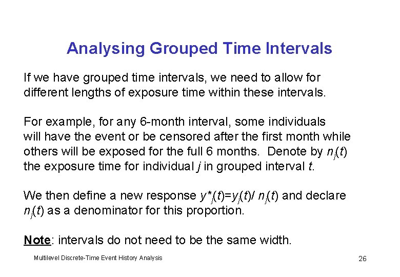
Analysing Grouped Time Intervals If we have grouped time intervals, we need to allow for different lengths of exposure time within these intervals. For example, for any 6 -month interval, some individuals will have the event or be censored after the first month while others will be exposed for the full 6 months. Denote by nj(t) the exposure time for individual j in grouped interval t. We then define a new response y*j(t)=yj(t)/ nj(t) and declare nj(t) as a denominator for this proportion. Note: intervals do not need to be the same width. Multilevel Discrete-Time Event History Analysis 26

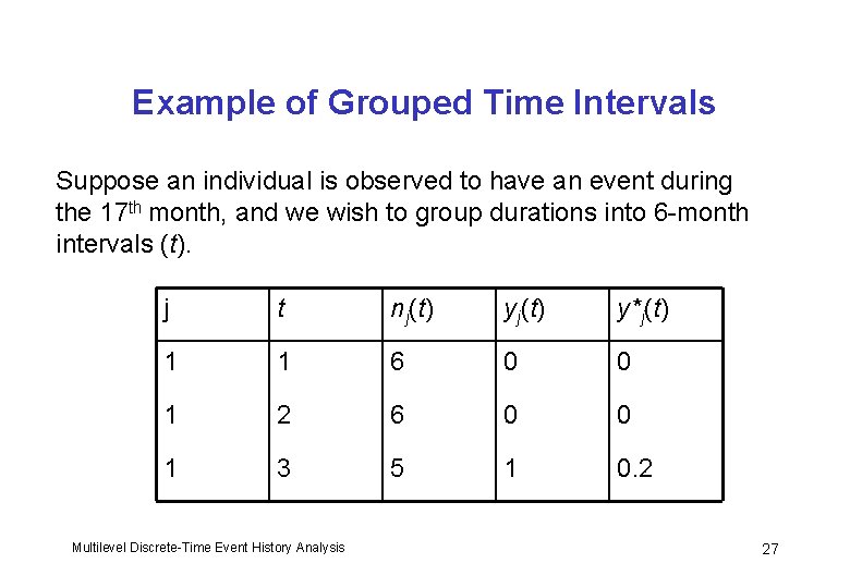
Example of Grouped Time Intervals Suppose an individual is observed to have an event during the 17 th month, and we wish to group durations into 6 -month intervals (t). j t nj(t) y*j(t) 1 1 6 0 0 1 2 6 0 0 1 3 5 1 0. 2 Multilevel Discrete-Time Event History Analysis 27

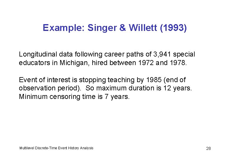
Example: Singer & Willett (1993) Longitudinal data following career paths of 3, 941 special educators in Michigan, hired between 1972 and 1978. Event of interest is stopping teaching by 1985 (end of observation period). So maximum duration is 12 years. Minimum censoring time is 7 years. Multilevel Discrete-Time Event History Analysis 28

Hazard and Survivor Functions Multilevel Discrete-Time Event History Analysis 29

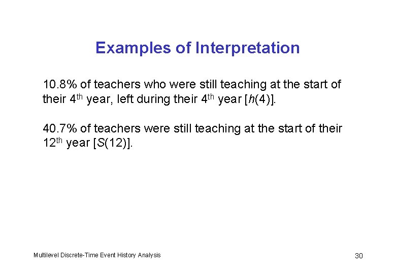
Examples of Interpretation 10. 8% of teachers who were still teaching at the start of their 4 th year, left during their 4 th year [h(4)]. 40. 7% of teachers were still teaching at the start of their 12 th year [S(12)]. Multilevel Discrete-Time Event History Analysis 30

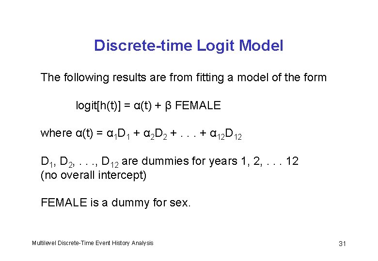
Discrete-time Logit Model The following results are from fitting a model of the form logit[h(t)] = α(t) + β FEMALE where α(t) = α 1 D 1 + α 2 D 2 +. . . + α 12 D 12 D 1, D 2, . . . , D 12 are dummies for years 1, 2, . . . 12 (no overall intercept) FEMALE is a dummy for sex. Multilevel Discrete-Time Event History Analysis 31

Results from Fitting Logit Model Multilevel Discrete-Time Event History Analysis 32

Unobserved Heterogeneity

Introduction Some individuals will be more at risk of experiencing an event than others, and it is unlikely that the reasons for this variability in the hazard will be fully captured by covariates. The presence of unobserved (or unobservable) individual-specific risk factors leads to unobserved heterogeneity in the hazard. Unobserved heterogeneity is also referred to as frailty, particularly in biostatistics (more ‘frail’ individuals have a higher mortality hazard). Multilevel Discrete-Time Event History Analysis 34

Consequences of Unobserved Heterogeneity If there are individual-specific unobserved factors that affect the hazard, the observed form of the hazard function at the aggregate population level will tend to be different from those at the individual level. Even if the hazards of individuals in a population are constant over time the aggregate population hazard may be time-dependent, typically decreasing. This may be explained by a selection effect operating on individuals. Multilevel Discrete-Time Event History Analysis 35

Selection Effect If a population is heterogeneous in its susceptibility to experiencing an event, high risk individuals will tend to have the event first, leaving lower risk individuals in the population. Therefore as t increases the population is increasingly depleted of those individuals most likely to experience the event, leading to a decrease in the population hazard. Because of this selection, we may see a decrease in the population hazard even if individual hazards are constant (or even increasing). Multilevel Discrete-Time Event History Analysis 36

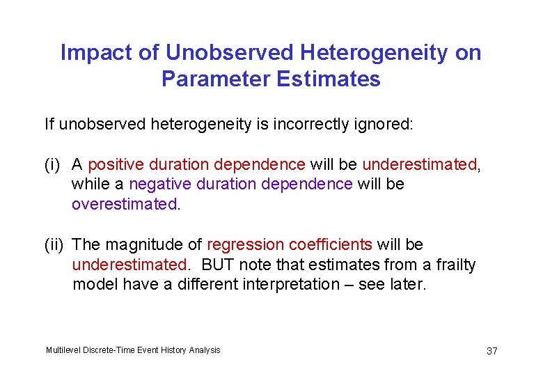
Impact of Unobserved Heterogeneity on Parameter Estimates If unobserved heterogeneity is incorrectly ignored: (i) A positive duration dependence will be underestimated, while a negative duration dependence will be overestimated. (ii) The magnitude of regression coefficients will be underestimated. BUT note that estimates from a frailty model have a different interpretation – see later. Multilevel Discrete-Time Event History Analysis 37

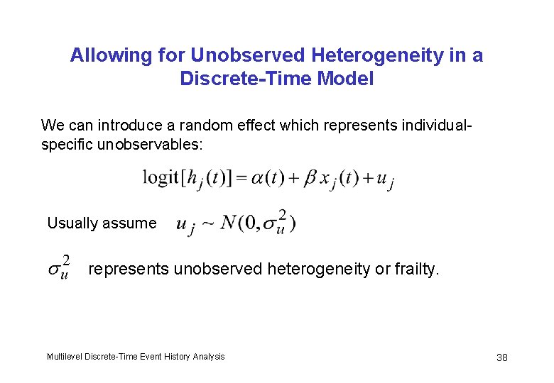
Allowing for Unobserved Heterogeneity in a Discrete-Time Model We can introduce a random effect which represents individualspecific unobservables: Usually assume represents unobserved heterogeneity or frailty. Multilevel Discrete-Time Event History Analysis 38

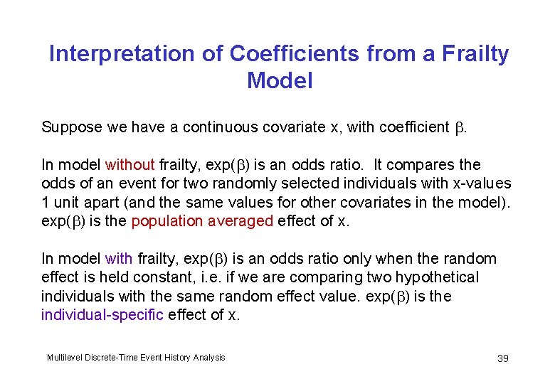
Interpretation of Coefficients from a Frailty Model Suppose we have a continuous covariate x, with coefficient . In model without frailty, exp( ) is an odds ratio. It compares the odds of an event for two randomly selected individuals with x-values 1 unit apart (and the same values for other covariates in the model). exp( ) is the population averaged effect of x. In model with frailty, exp( ) is an odds ratio only when the random effect is held constant, i. e. if we are comparing two hypothetical individuals with the same random effect value. exp( ) is the individual-specific effect of x. Multilevel Discrete-Time Event History Analysis 39

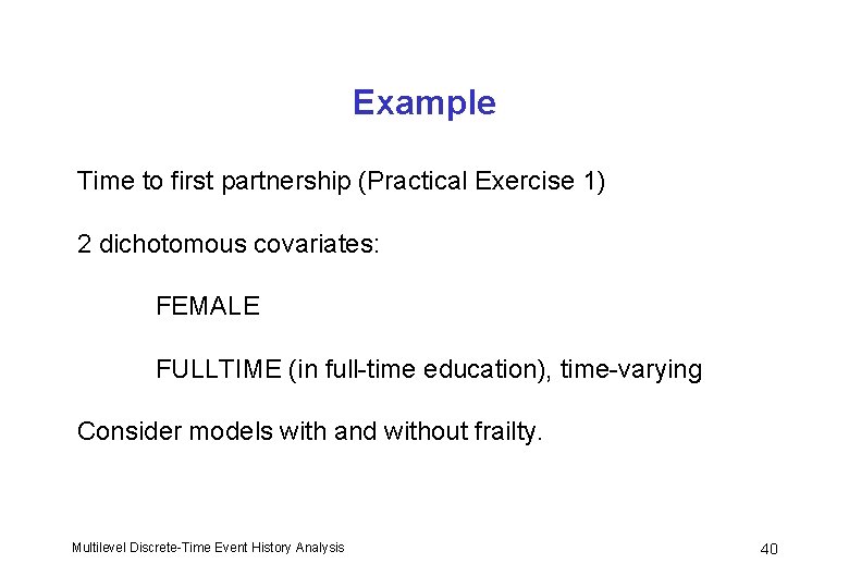
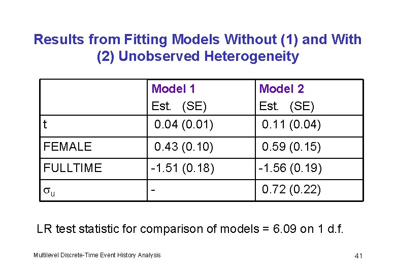
Example Time to first partnership (Practical Exercise 1) 2 dichotomous covariates: FEMALE FULLTIME (in full-time education), time-varying Consider models with and without frailty. Multilevel Discrete-Time Event History Analysis 40

Results from Fitting Models Without (1) and With (2) Unobserved Heterogeneity t Model 1 Est. (SE) 0. 04 (0. 01) Model 2 Est. (SE) 0. 11 (0. 04) FEMALE 0. 43 (0. 10) 0. 59 (0. 15) FULLTIME -1. 51 (0. 18) -1. 56 (0. 19) u - 0. 72 (0. 22) LR test statistic for comparison of models = 6. 09 on 1 d. f. Multilevel Discrete-Time Event History Analysis 41

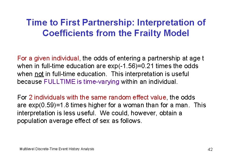
Time to First Partnership: Interpretation of Coefficients from the Frailty Model For a given individual, the odds of entering a partnership at age t when in full-time education are exp(-1. 56)=0. 21 times the odds when not in full-time education. This interpretation is useful because FULLTIME is time-varying within an individual. For 2 individuals with the same random effect value, the odds are exp(0. 59)=1. 8 times higher for a woman than for a man. This interpretation is less useful. We could, however, obtain a population average effect of sex as follows. Multilevel Discrete-Time Event History Analysis 42

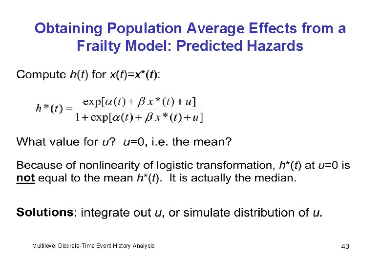
Obtaining Population Average Effects from a Frailty Model: Predicted Hazards Multilevel Discrete-Time Event History Analysis 43

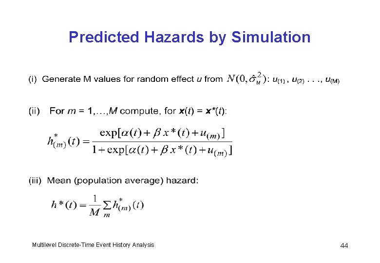
Predicted Hazards by Simulation Multilevel Discrete-Time Event History Analysis 44

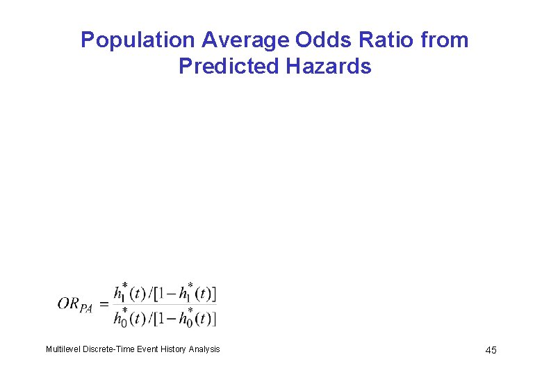
Population Average Odds Ratio from Predicted Hazards Multilevel Discrete-Time Event History Analysis 45

Estimation of Model with Unobserved Heterogeneity • Estimate using any software for random effects (multilevel) logit models. Options include: – SAS (proc nlmixed), Stata (xtlogit), a. ML (all use numerical quadrature) – MLwi. N (quasi-likelihood, MCMC) – Win. BUGS (MCMC) Multilevel Discrete-Time Event History Analysis 46

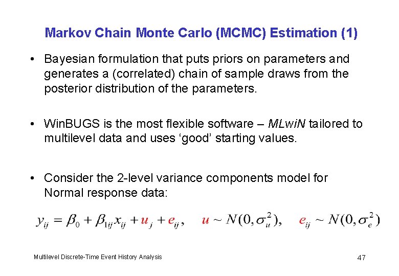
Markov Chain Monte Carlo (MCMC) Estimation (1) • Bayesian formulation that puts priors on parameters and generates a (correlated) chain of sample draws from the posterior distribution of the parameters. • Win. BUGS is the most flexible software – MLwi. N tailored to multilevel data and uses ‘good’ starting values. • Consider the 2 -level variance components model for Normal response data: Multilevel Discrete-Time Event History Analysis 47

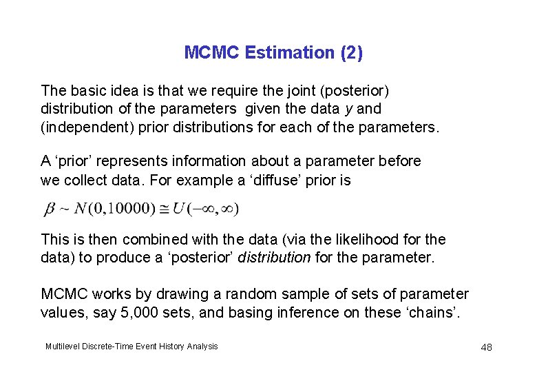
MCMC Estimation (2) The basic idea is that we require the joint (posterior) distribution of the parameters given the data y and (independent) prior distributions for each of the parameters. A ‘prior’ represents information about a parameter before we collect data. For example a ‘diffuse’ prior is This is then combined with the data (via the likelihood for the data) to produce a ‘posterior’ distribution for the parameter. MCMC works by drawing a random sample of sets of parameter values, say 5, 000 sets, and basing inference on these ‘chains’. Multilevel Discrete-Time Event History Analysis 48

MCMC Estimation (3) At iteration n we want to sample from the posterior distribution of each parameter in turn. If we can write down an analytical expression for the posterior – as is the case for Normal models - then Gibbs sampling is available and efficient. Otherwise we need an alternative – MLwi. N uses Metropolis-Hastings sampling, e. g. for binary response models. Multilevel Discrete-Time Event History Analysis 49

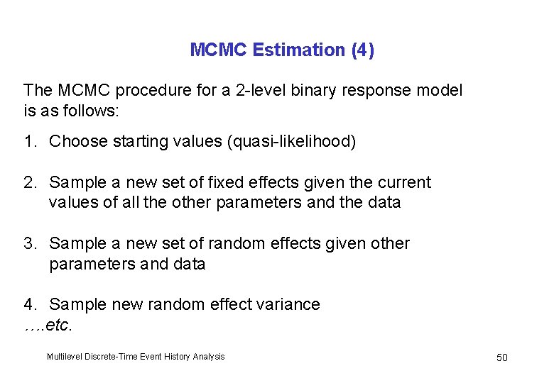
MCMC Estimation (4) The MCMC procedure for a 2 -level binary response model is as follows: 1. Choose starting values (quasi-likelihood) 2. Sample a new set of fixed effects given the current values of all the other parameters and the data 3. Sample a new set of random effects given other parameters and data 4. Sample new random effect variance …. etc. Multilevel Discrete-Time Event History Analysis 50

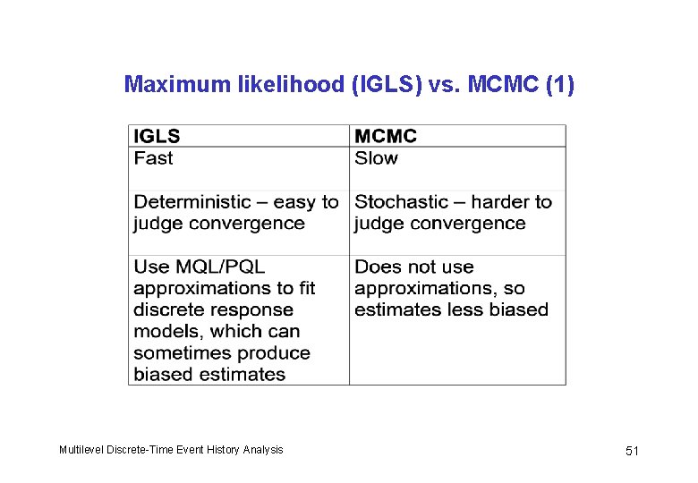
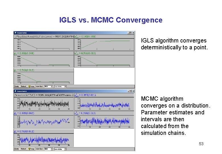
Maximum likelihood (IGLS) vs. MCMC (1) Multilevel Discrete-Time Event History Analysis 51

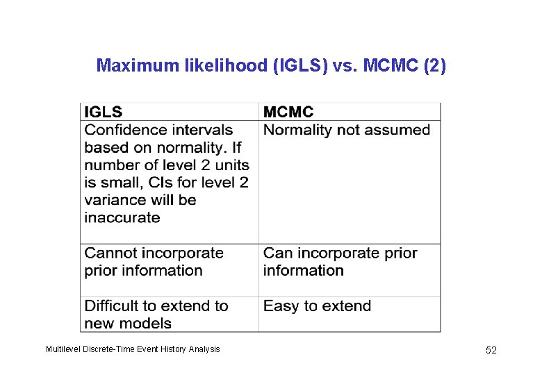
Maximum likelihood (IGLS) vs. MCMC (2) Multilevel Discrete-Time Event History Analysis 52

IGLS vs. MCMC Convergence IGLS algorithm converges deterministically to a point. MCMC algorithm converges on a distribution. Parameter estimates and intervals are then calculated from the simulation chains. Multilevel Discrete-Time Event History Analysis 53

Obtaining Parameter Estimates in MCMC • For each parameter, we have a large number of simulated draws called a chain. The period when the chains are settling down (converging) to the posterior distribution is called the burn-in; these samples are discarded. • Summary statistics of the chains can then be calculated. Means and standard deviations (analogous to frequentist standard errors) are shown in the MLwi. N Equations window. • 95% interval estimates can be obtained by taking the 2. 5% and 97. 5% points of the ordered chain values. Multilevel Discrete-Time Event History Analysis 54

Other MCMC Issues • By default MLwi. N uses flat, uninformative priors (see p. 5 of MCMC Estimation in MLwi. N, downloadable from www. cmm. bris. ac. uk/MLwi. N/download/manuals. shtml) • To specify informative priors, see Ch. 6 • For model comparison in MCMC using the DIC statistics, see Ch. 3 & 4 • For description of MCMC algorithms used in MLwi. N, see Ch. 2 Multilevel Discrete-Time Event History Analysis 55

When to Consider using MCMC in MLwi. N • Discrete response data (categorical, counts). PQL often gives quick and accurate estimates but a good idea to check against MCMC, especially if you have small clusters. • If you have few level 2 units and want to make accurate inferences about level 2 variances. • Some advanced models only estimated using MCMC (e. g. multilevel factor analysis) • Some models can be fitted more easily using MCMC (e. g. multiple imputation, cross-classified models) Multilevel Discrete-Time Event History Analysis 56

Modelling Recurrent Events

Examples of Recurrent Events Many types of event can occur more than once to an individual. Define an episode as the time between the start of the ‘risk’ period and the occurrence of an event or censoring. Examples Employment episode: duration from starting a new job to leaving that job. Marriage episode: duration of a marriage. Multilevel Discrete-Time Event History Analysis 58

Problem with Analysing Recurrent Events We cannot assume that the durations of episodes from the same individual are independent. There may be unobserved individual-specific factors (i. e. constant across episodes) which affect the hazard of an event for all episodes. Presence of such unobservables, and failure to account for them in the model, will lead to correlation between the durations of episodes from the same individual. Multilevel Discrete-Time Event History Analysis 59

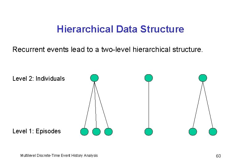
Hierarchical Data Structure Recurrent events lead to a two-level hierarchical structure. Level 2: Individuals Level 1: Episodes Multilevel Discrete-Time Event History Analysis 60

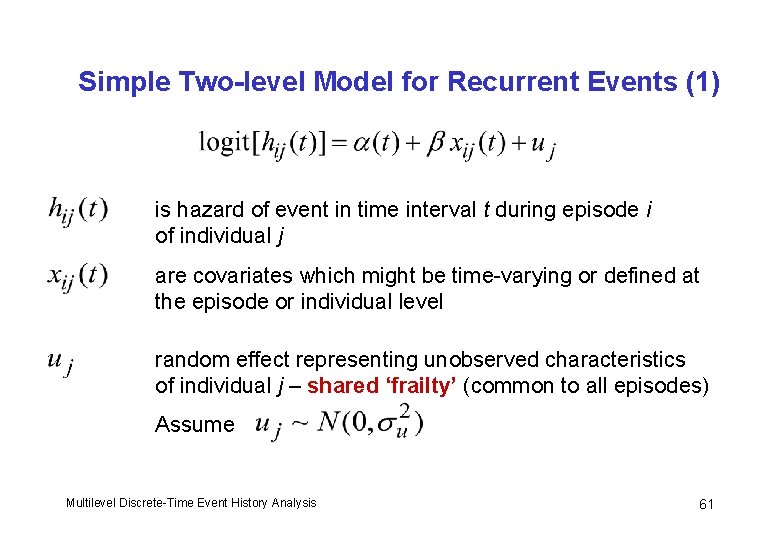
Simple Two-level Model for Recurrent Events (1) is hazard of event in time interval t during episode i of individual j are covariates which might be time-varying or defined at the episode or individual level random effect representing unobserved characteristics of individual j – shared ‘frailty’ (common to all episodes) Assume Multilevel Discrete-Time Event History Analysis 61

Simple Two-level Model for Recurrent Events (2) • The model for recurrent events is essentially the same as the model for unobserved heterogeneity, and is therefore estimated in exactly the same way. • Recurrent events allow better identification of the random effect variance. • The expansion of data to discrete-time format is carried out for each episode within an individual. Multilevel Discrete-Time Event History Analysis 62

Episode-specific Effects We can allow the duration and covariate effects to vary between episodes. E. g. we might expect factors affecting the timing of the first event to differ from those affecting timing of subsequent events (or the same factors to have different effects). Include dummy variable(s) for order of the event and interact with t and covariates. Multilevel Discrete-Time Event History Analysis 63

Example Repeated birth intervals for Hutterite women, a natural fertility (no contraceptive use) population in North America. Data on 944 birth intervals from 159 women. Interval is duration between a birth and conception of next child. Only closed intervals (i. e. ending in a conception before the survey). Long open intervals may be due to primary or secondary sterility. Therefore there is no censoring. Multilevel Discrete-Time Event History Analysis 64

Duration and Covariates Duration of a birth interval is represented by a categorical variable (in a piecewise constant hazards model): MONTH Month of exposure to risk of conception [<6, 6 -11, 12 -23, 24 -35, 36+ (ref. )] Consider one covariate: AGE Age at start of birth interval (years) Multilevel Discrete-Time Event History Analysis 65

Results Multilevel Discrete-Time Event History Analysis 66

Random Coefficient Models The model we have considered so far assumes that unobserved heterogeneity is constant. Using multilevel modelling terminology, this model is a random intercept model. The form of the hazard is assumed the same across individuals, but is shifted up or down by an amount uj on the logit scale. The duration and covariate effects are assumed to be the same for each individual. To test these assumptions, we can consider random coefficient models (called random slope models for continuous covariates with linear effects). Note, however, that there may be insufficient information to estimate random coefficients if the number of individuals with recurrent events is small. Multilevel Discrete-Time Event History Analysis 67

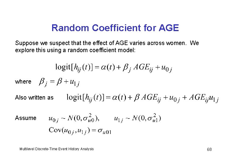
Random Coefficient for AGE Suppose we suspect that the effect of AGE varies across women. We explore this using a random coefficient model: where Also written as Assume Multilevel Discrete-Time Event History Analysis 68

Graphical Representation of a Random Coefficient Model For any time interval t: Multilevel Discrete-Time Event History Analysis 69

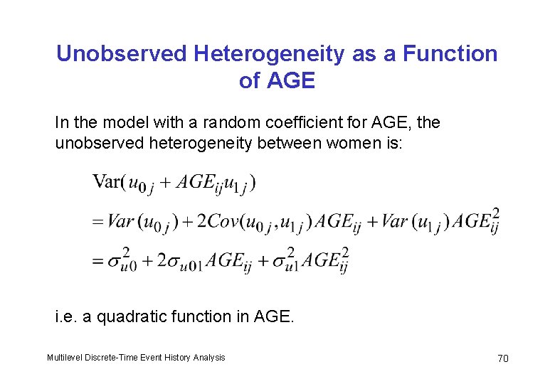
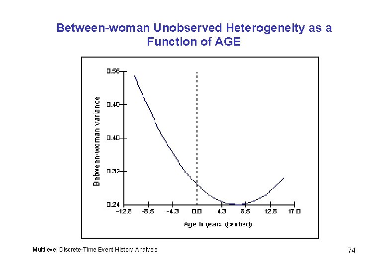
Unobserved Heterogeneity as a Function of AGE In the model with a random coefficient for AGE, the unobserved heterogeneity between women is: i. e. a quadratic function in AGE. Multilevel Discrete-Time Event History Analysis 70

Results from Random Coefficient Model (AGE centred around mean) Multilevel Discrete-Time Event History Analysis 71

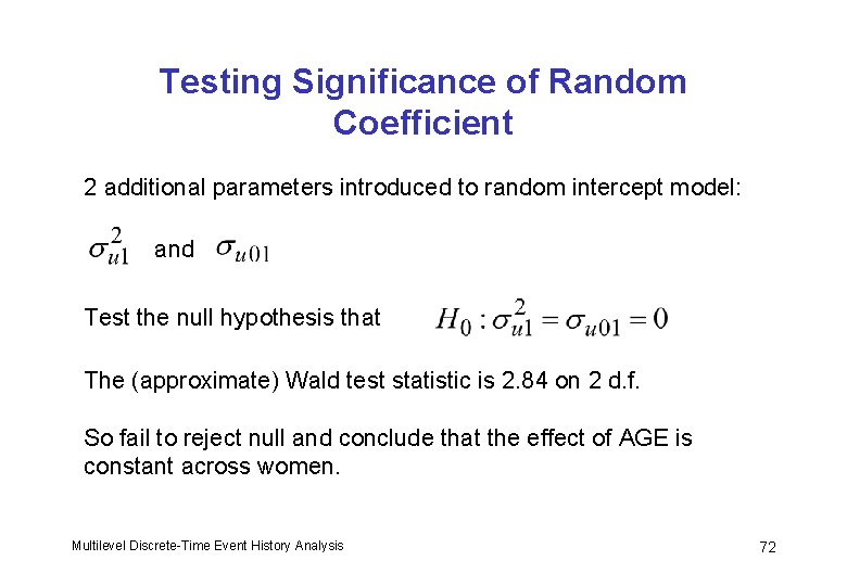
Testing Significance of Random Coefficient 2 additional parameters introduced to random intercept model: and Test the null hypothesis that The (approximate) Wald test statistic is 2. 84 on 2 d. f. So fail to reject null and conclude that the effect of AGE is constant across women. Multilevel Discrete-Time Event History Analysis 72

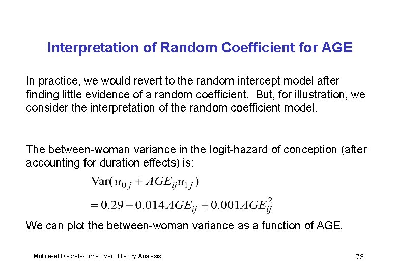
Interpretation of Random Coefficient for AGE In practice, we would revert to the random intercept model after finding little evidence of a random coefficient. But, for illustration, we consider the interpretation of the random coefficient model. The between-woman variance in the logit-hazard of conception (after accounting for duration effects) is: We can plot the between-woman variance as a function of AGE. Multilevel Discrete-Time Event History Analysis 73

Between-woman Unobserved Heterogeneity as a Function of AGE Multilevel Discrete-Time Event History Analysis 74

Multiple States

States in Event Histories In the models we have considered so far, there is a single event of interest. We model the duration to this event from the point at which an individual becomes “at risk”. We can think of this as the duration spent in the same state. E. g. in a study of marital dissolution we model the duration in the marriage state. In a study of birth intervals we model the duration spent in the non-pregnant state (up to age 45 say). Multilevel Discrete-Time Event History Analysis 76

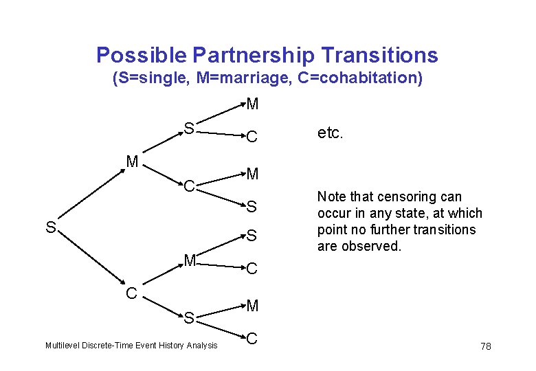
Multiple States Usually individuals will move in and out of different states over time, and we wish to model these transitions. Examples Partnership states: marriage, cohabitation, single (unpartnered) Employment states: employed, unemployed, out of the labour market Multilevel Discrete-Time Event History Analysis 77

Possible Partnership Transitions (S=single, M=marriage, C=cohabitation) M S M C C M S S S M C S Multilevel Discrete-Time Event History Analysis etc. Note that censoring can occur in any state, at which point no further transitions are observed. C M C 78

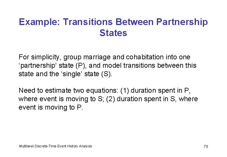
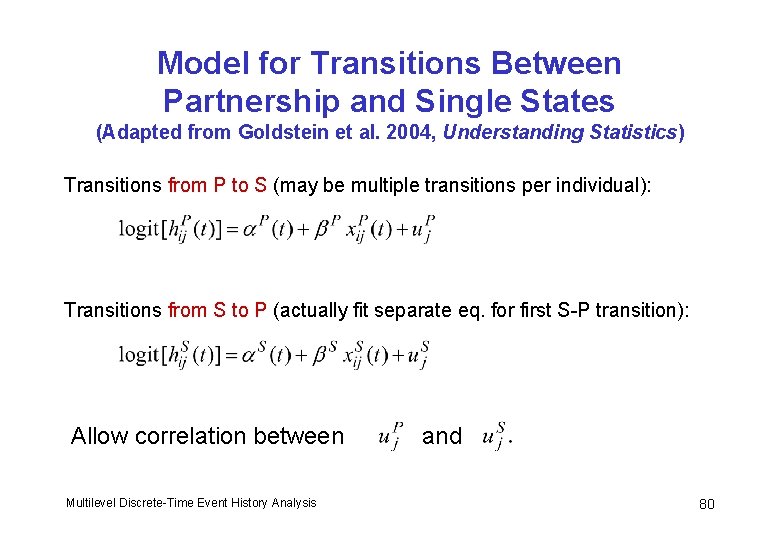
Example: Transitions Between Partnership States For simplicity, group marriage and cohabitation into one ‘partnership’ state (P), and model transitions between this state and the ‘single’ state (S). Need to estimate two equations: (1) duration spent in P, where event is moving to S; (2) duration spent in S, where event is moving to P. Multilevel Discrete-Time Event History Analysis 79

Model for Transitions Between Partnership and Single States (Adapted from Goldstein et al. 2004, Understanding Statistics) Transitions from P to S (may be multiple transitions per individual): Transitions from S to P (actually fit separate eq. for first S-P transition): Allow correlation between Multilevel Discrete-Time Event History Analysis and 80

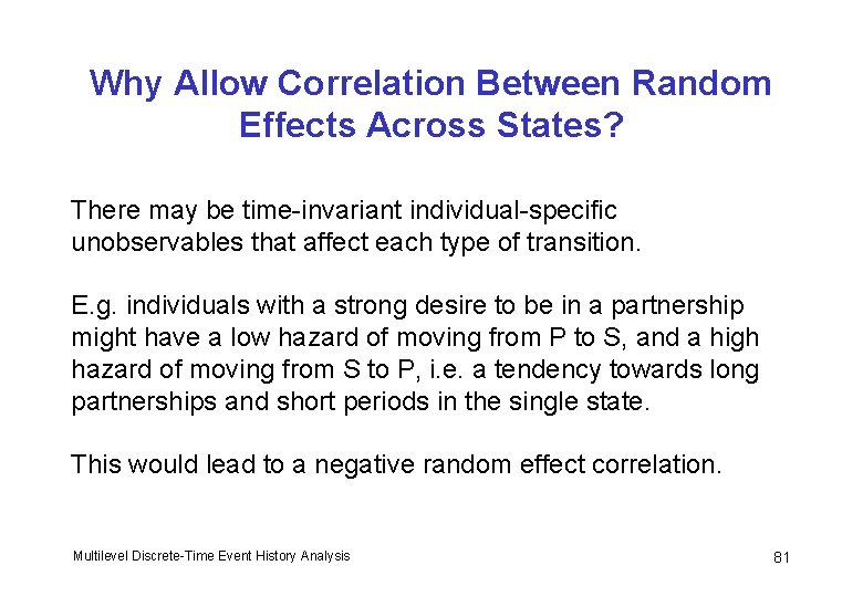
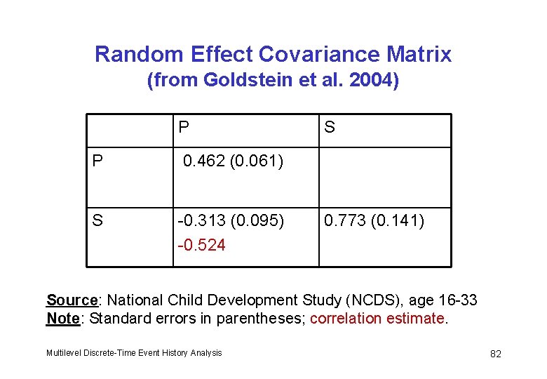
Why Allow Correlation Between Random Effects Across States? There may be time-invariant individual-specific unobservables that affect each type of transition. E. g. individuals with a strong desire to be in a partnership might have a low hazard of moving from P to S, and a high hazard of moving from S to P, i. e. a tendency towards long partnerships and short periods in the single state. This would lead to a negative random effect correlation. Multilevel Discrete-Time Event History Analysis 81

Random Effect Covariance Matrix (from Goldstein et al. 2004) P P 0. 462 (0. 061) S -0. 313 (0. 095) -0. 524 S 0. 773 (0. 141) Source: National Child Development Study (NCDS), age 16 -33 Note: Standard errors in parentheses; correlation estimate. Multilevel Discrete-Time Event History Analysis 82

Interpretation of Random Effect Correlation (Men only) The estimated correlation of – 0. 524 implies that there is a moderate negative association between the duration in a partnership and the duration spent without a partner. We can, tentatively, classify men as long partnership/ short-time single or short partnership/ long-time single. Multilevel Discrete-Time Event History Analysis 83

Estimation of a Multiple State Model • Specify a single equation model with dummy variables for each state. Interact dummies with duration and covariates to obtain state-specific duration and covariate effects. • Allow coefficient of each dummy to vary and covary randomly across individuals. Multilevel Discrete-Time Event History Analysis 84

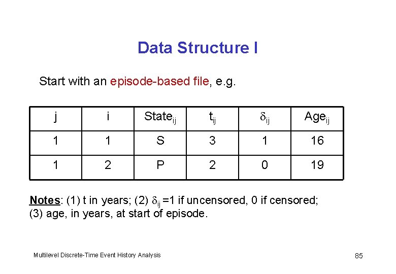
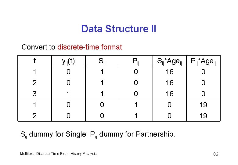
Data Structure I Start with an episode-based file, e. g. j i Stateij tij ij Ageij 1 1 S 3 1 16 1 2 P 2 0 19 Notes: (1) t in years; (2) ij =1 if uncensored, 0 if censored; (3) age, in years, at start of episode. Multilevel Discrete-Time Event History Analysis 85

Data Structure II Convert to discrete-time format: t 1 2 3 yij(t) 0 0 1 Sij 1 1 1 Pij 0 0 0 Sij*Ageij 16 16 16 Pij*Ageij 0 0 0 1 2 0 0 1 1 0 0 19 19 Sij dummy for Single, Pij dummy for Partnership. Multilevel Discrete-Time Event History Analysis 86

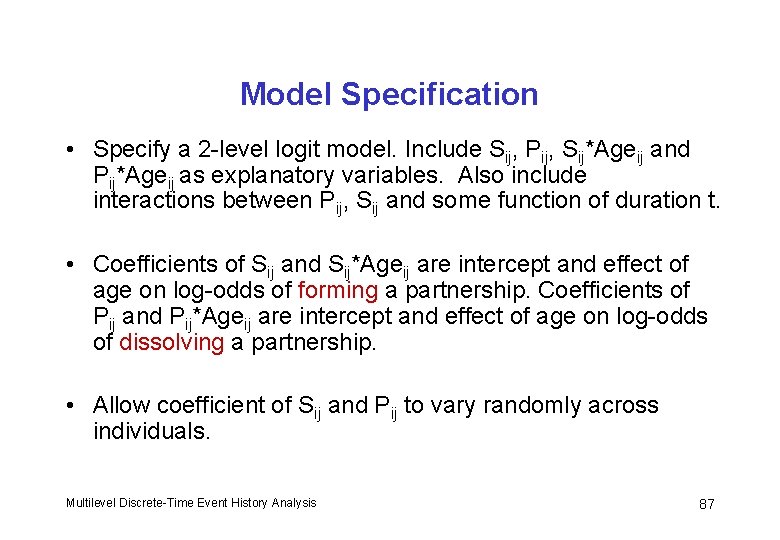
Model Specification • Specify a 2 -level logit model. Include Sij, Pij, Sij*Ageij and Pij*Ageij as explanatory variables. Also include interactions between Pij, Sij and some function of duration t. • Coefficients of Sij and Sij*Ageij are intercept and effect of age on log-odds of forming a partnership. Coefficients of Pij and Pij*Ageij are intercept and effect of age on log-odds of dissolving a partnership. • Allow coefficient of Sij and Pij to vary randomly across individuals. Multilevel Discrete-Time Event History Analysis 87

Competing Risks

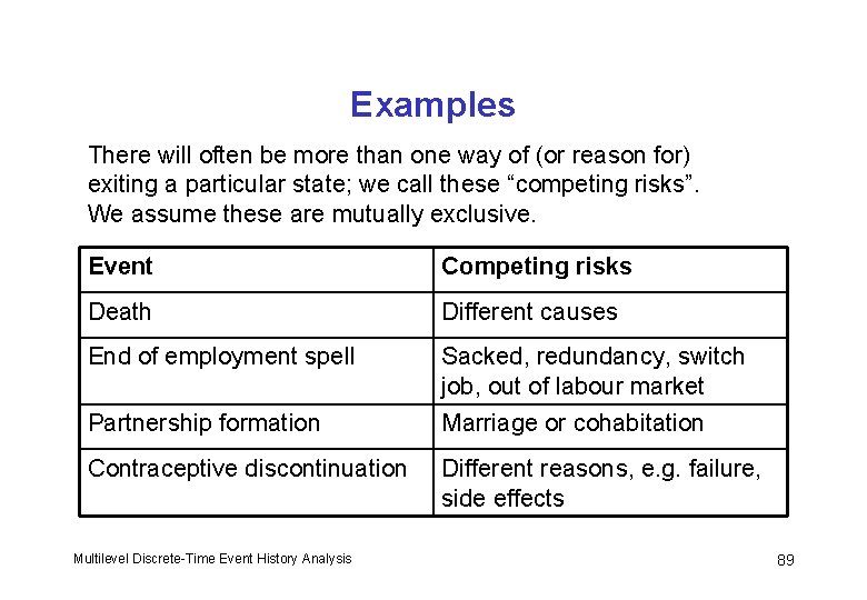
Examples There will often be more than one way of (or reason for) exiting a particular state; we call these “competing risks”. We assume these are mutually exclusive. Event Competing risks Death Different causes End of employment spell Sacked, redundancy, switch job, out of labour market Partnership formation Marriage or cohabitation Contraceptive discontinuation Different reasons, e. g. failure, side effects Multilevel Discrete-Time Event History Analysis 89

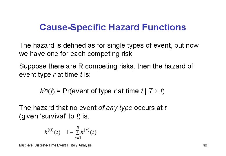
Cause-Specific Hazard Functions The hazard is defined as for single types of event, but now we have one for each competing risk. Suppose there are R competing risks, then the hazard of event type r at time t is: h(r)(t) = Pr(event of type r at time t | T t) The hazard that no event of any type occurs at t (given ‘survival’ to t) is: Multilevel Discrete-Time Event History Analysis 90

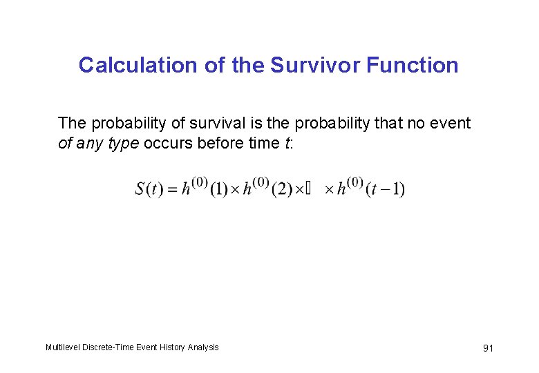
Calculation of the Survivor Function The probability of survival is the probability that no event of any type occurs before time t: Multilevel Discrete-Time Event History Analysis 91

Modelling Approaches I In discrete time, we can distinguish between two main modelling approaches: (1) Model the cause-specific hazards simultaneously using a multinomial logistic model E. g. for partnership formation, estimate 2 contrasts: marriage vs. single (“no event”), cohabitation vs. single. (The remaining contrast, marriage vs. cohabitation, may be estimated from the other two. ) c. f. Multiple decrement life table Multilevel Discrete-Time Event History Analysis 92

Modelling Approaches II (2) Model each competing risk separately, treating all other events as censored E. g. for partnership formation, estimate 2 separate binary logistic models: (i) Model hazard of marriage, treating transitions to cohabitation as censored; (ii) Model hazard of cohabitation, treating transitions to marriage as censored. c. f. Associated single decrement life table Multilevel Discrete-Time Event History Analysis 93

Modelling Approaches III § Rates estimated using approach (2) represent the underlying (or theoretical) risk of a particular event in the absence of all other risks. E. g. “What would be the risk of dying from cancer if there were no other causes of death? ” § Useful for comparing rates across time or populations. E. g. Comparison of death rates due to cancer in 1900 and 1990, adjusting for changes in life expectancy. Multilevel Discrete-Time Event History Analysis 94

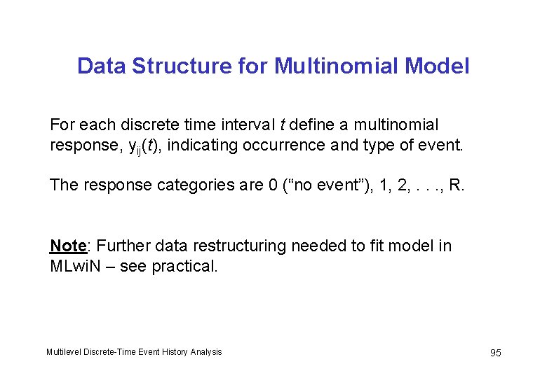
Data Structure for Multinomial Model For each discrete time interval t define a multinomial response, yij(t), indicating occurrence and type of event. The response categories are 0 (“no event”), 1, 2, . . . , R. Note: Further data restructuring needed to fit model in MLwi. N – see practical. Multilevel Discrete-Time Event History Analysis 95

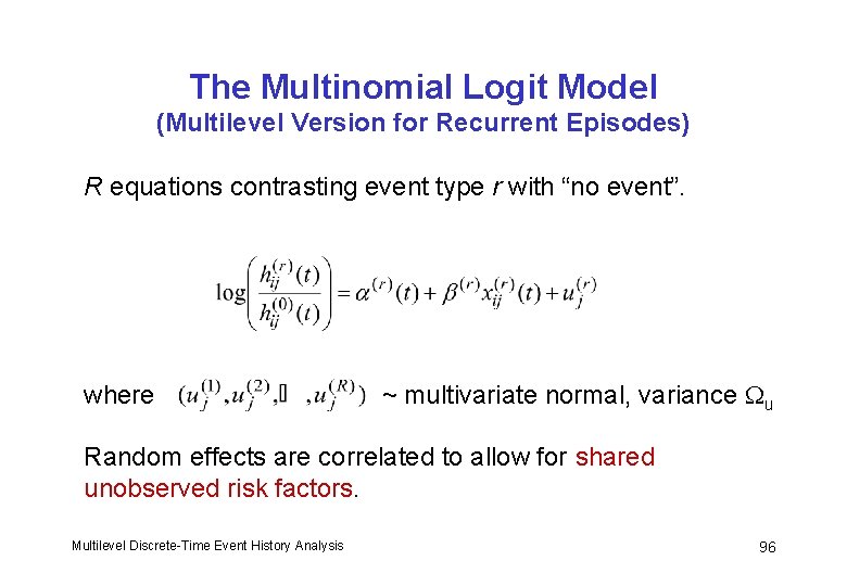
The Multinomial Logit Model (Multilevel Version for Recurrent Episodes) R equations contrasting event type r with “no event”. where ~ multivariate normal, variance u Random effects are correlated to allow for shared unobserved risk factors. Multilevel Discrete-Time Event History Analysis 96

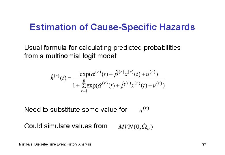
Estimation of Cause-Specific Hazards Usual formula for calculating predicted probabilities from a multinomial logit model: Need to substitute some value for Could simulate values from Multilevel Discrete-Time Event History Analysis 97

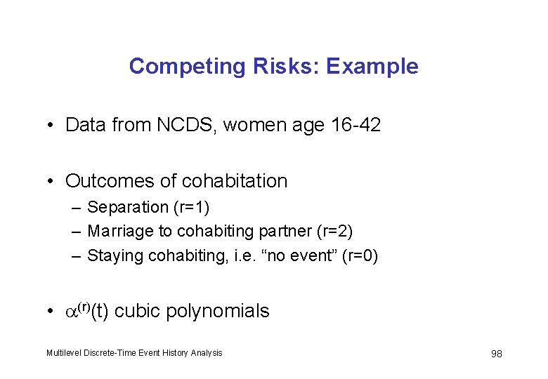
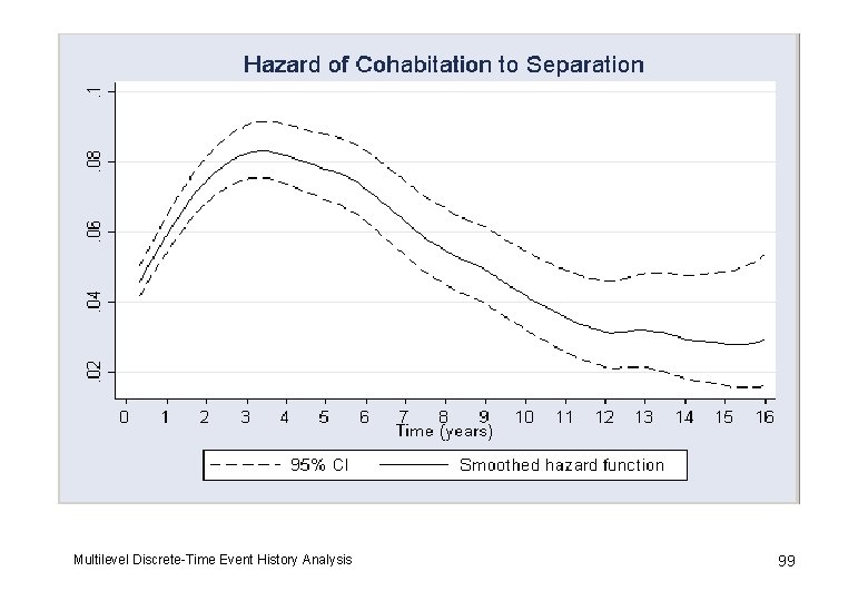
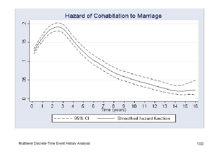
Competing Risks: Example • Data from NCDS, women age 16 -42 • Outcomes of cohabitation – Separation (r=1) – Marriage to cohabiting partner (r=2) – Staying cohabiting, i. e. “no event” (r=0) • (r)(t) cubic polynomials Multilevel Discrete-Time Event History Analysis 98

Multilevel Discrete-Time Event History Analysis 99

Multilevel Discrete-Time Event History Analysis 100

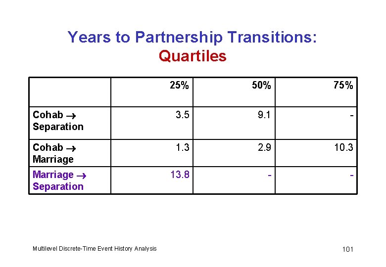
Years to Partnership Transitions: Quartiles 25% 50% 75% Cohab Separation 3. 5 9. 1 - Cohab Marriage 1. 3 2. 9 10. 3 13. 8 - - Marriage Separation Multilevel Discrete-Time Event History Analysis 101

Cohabitation Outcomes: Selected Results Multilevel Discrete-Time Event History Analysis 102

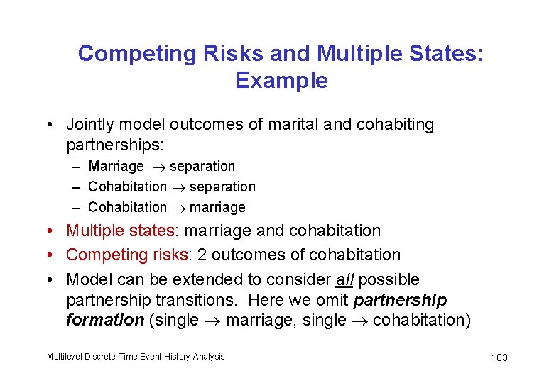
Competing Risks and Multiple States: Example • Jointly model outcomes of marital and cohabiting partnerships: – Marriage separation – Cohabitation marriage • Multiple states: marriage and cohabitation • Competing risks: 2 outcomes of cohabitation • Model can be extended to consider all possible partnership transitions. Here we omit partnership formation (single marriage, single cohabitation) Multilevel Discrete-Time Event History Analysis 103

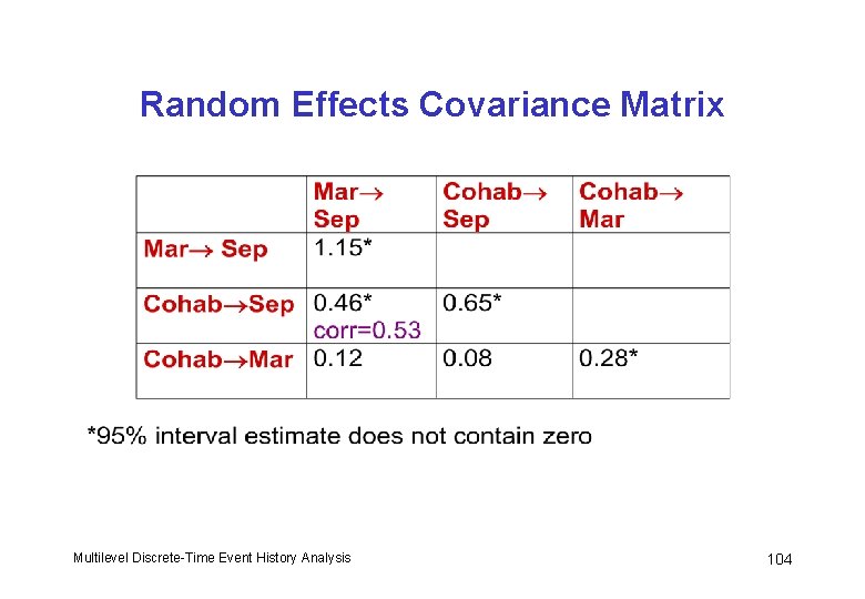
Random Effects Covariance Matrix Multilevel Discrete-Time Event History Analysis 104

Interpretation of Random Effect Correlation between random effects for dissolution of marriage and cohabitation is estimated as 0. 53. Women with a high (low) risk of separation from marriage tend also to have a high (low) risk of separation from cohabitation. Multilevel Discrete-Time Event History Analysis 105

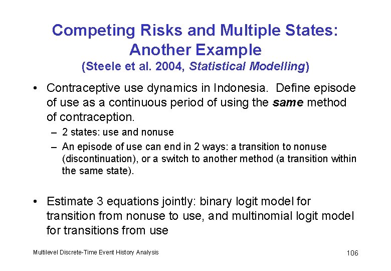
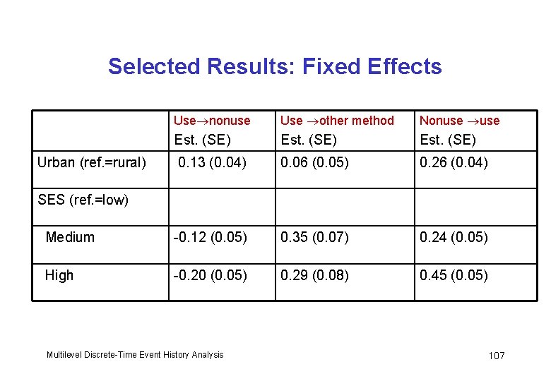
Competing Risks and Multiple States: Another Example (Steele et al. 2004, Statistical Modelling) • Contraceptive use dynamics in Indonesia. Define episode of use as a continuous period of using the same method of contraception. – 2 states: use and nonuse – An episode of use can end in 2 ways: a transition to nonuse (discontinuation), or a switch to another method (a transition within the same state). • Estimate 3 equations jointly: binary logit model for transition from nonuse to use, and multinomial logit model for transitions from use Multilevel Discrete-Time Event History Analysis 106

Selected Results: Fixed Effects Use nonuse Use other method Nonuse Est. (SE) 0. 13 (0. 04) 0. 06 (0. 05) 0. 26 (0. 04) Medium -0. 12 (0. 05) 0. 35 (0. 07) 0. 24 (0. 05) High -0. 20 (0. 05) 0. 29 (0. 08) 0. 45 (0. 05) Urban (ref. =rural) SES (ref. =low) Multilevel Discrete-Time Event History Analysis 107

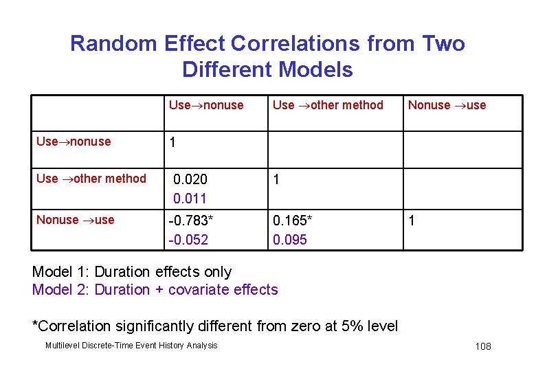
Random Effect Correlations from Two Different Models Use nonuse Use other method Nonuse use 1 0. 020 0. 011 1 -0. 783* -0. 052 0. 165* 0. 095 1 Model 1: Duration effects only Model 2: Duration + covariate effects *Correlation significantly different from zero at 5% level Multilevel Discrete-Time Event History Analysis 108

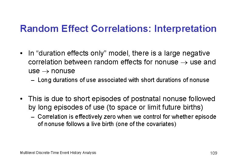
Random Effect Correlations: Interpretation • In “duration effects only” model, there is a large negative correlation between random effects for nonuse and use nonuse – Long durations of use associated with short durations of nonuse • This is due to short episodes of postnatal nonuse followed by long episodes of use (to space or limit future births) – Correlation is effectively zero when we control for whether episode of nonuse follows a live birth (one of the covariates) Multilevel Discrete-Time Event History Analysis 109

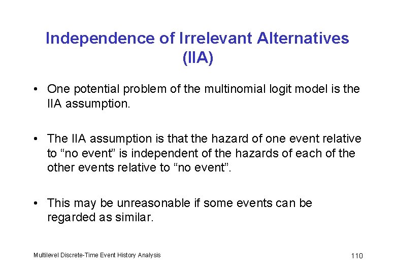
Independence of Irrelevant Alternatives (IIA) • One potential problem of the multinomial logit model is the IIA assumption. • The IIA assumption is that the hazard of one event relative to “no event” is independent of the hazards of each of the other events relative to “no event”. • This may be unreasonable if some events can be regarded as similar. Multilevel Discrete-Time Event History Analysis 110

Example: Partnership Formation (Marriage vs. Cohabitation) • Under IIA, assume the hazard of cohabitation vs. staying single is uncorrelated with the hazard of marriage vs. staying single. • E. g. If there is something unobserved (not in X’s) that made marriage unfeasible, we assume those who would have married distribute themselves between cohabitation and single in the same proportions as those who originally chose not to marry. • But as marriage and cohabitation are similar in some respects, we might expect those who are precluded from marriage to be more likely to cohabit rather than remain single (Hill, Axinn and Thornton, 1993, Sociological Methodology). Multilevel Discrete-Time Event History Analysis 111

IIA: Solutions • The random effects multinomial logit offers some protection against the IIA assumption. The correlation between the cause-specific random effects allows for similarity between alternatives due to time-invariant individual characteristics. It does not control for unmeasured factors that vary across episodes (e. g. whether respondent or partner is already married). • Another approach is to use a multinomial probit model (e. g. using a. ML). Or nested logit model (Hill et al. 1993). Multilevel Discrete-Time Event History Analysis 112

Multiple Processes

Endogeneity (1) Consider a 2 -level random effects model for a Normal response: One assumption of the model is that the predictors xij are uncorrelated with the residuals (uj, eij), i. e. we assume that xij are exogenous. This may too strong an assumption for some predictors, particularly “choice” variables. Multilevel Discrete-Time Event History Analysis 114

Endogeneity (2) E. g. suppose yij is birth weight of child i of woman j, and zij (an element of xij) is number of antenatal visits during pregnancy. Some of the factors that influence birth weight may also influence the uptake of antenatal care; these may be characteristics of the particular pregnancy (e. g. woman’s health during pregnancy) or of the woman (health-related behaviour). Some of these may be unobserved. i. e. y and z are to some extent jointly determined. z is said to be endogenous. This will lead to correlation between z and u and/or e, and a biased estimate of the coefficient of z. Multilevel Discrete-Time Event History Analysis 115

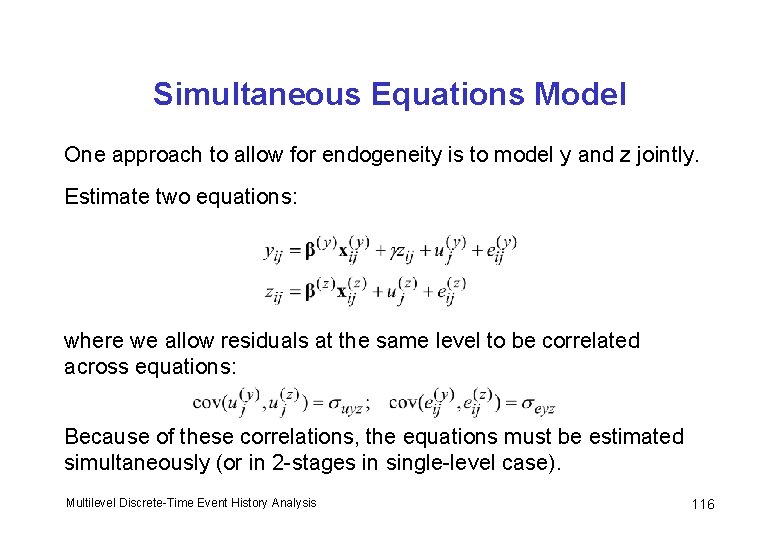
Simultaneous Equations Model One approach to allow for endogeneity is to model y and z jointly. Estimate two equations: where we allow residuals at the same level to be correlated across equations: Because of these correlations, the equations must be estimated simultaneously (or in 2 -stages in single-level case). Multilevel Discrete-Time Event History Analysis 116

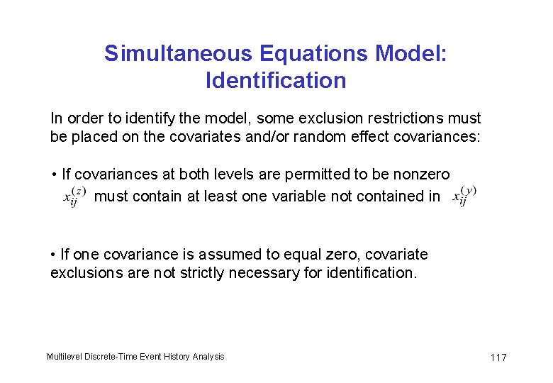
Simultaneous Equations Model: Identification In order to identify the model, some exclusion restrictions must be placed on the covariates and/or random effect covariances: • If covariances at both levels are permitted to be nonzero must contain at least one variable not contained in • If one covariance is assumed to equal zero, covariate exclusions are not strictly necessary for identification. Multilevel Discrete-Time Event History Analysis 117

Simultaneous Equations Model: Estimation Treat (yij, zij) as a bivariate response, and estimate multilevel bivariate response model (e. g. in MLwi. N, Chapter 14 in manual). Model can be extended to handle categorical responses (e. g. bivariate probit model) or mixture of Normal and categorical responses. MLwi. N can handle mixture of binary and Normal, and binary and multinomial (if zero covariance assumed at lowest level). a. ML can handle other mixtures. Multilevel Discrete-Time Event History Analysis 118

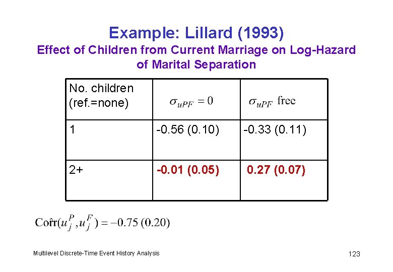
Simultaneous Equations Model for Correlated Event Histories (1) Suppose y is a duration variable and z is either also a duration or the outcome of an event history. E. g. (Lillard 1993; Lillard and Waite, 1993) yij is duration of marriage i of person j zij(t) is number of children from marriage i at time t (outcome of birth history) The unobserved individual characteristics that affect hazard of marital separation may be correlated with those that affect hazard of birth (or conception) during marriage. Multilevel Discrete-Time Event History Analysis 119

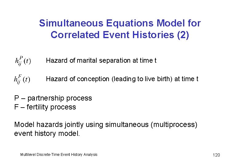
Simultaneous Equations Model for Correlated Event Histories (2) Hazard of marital separation at time t Hazard of conception (leading to live birth) at time t P – partnership process F – fertility process Model hazards jointly using simultaneous (multiprocess) event history model. Multilevel Discrete-Time Event History Analysis 120

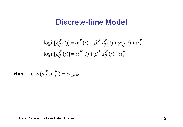
Discrete-time Model where Multilevel Discrete-Time Event History Analysis 121

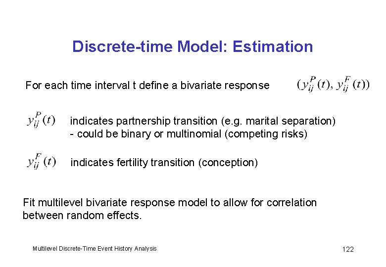
Discrete-time Model: Estimation For each time interval t define a bivariate response indicates partnership transition (e. g. marital separation) - could be binary or multinomial (competing risks) indicates fertility transition (conception) Fit multilevel bivariate response model to allow for correlation between random effects. Multilevel Discrete-Time Event History Analysis 122

Example: Lillard (1993) Effect of Children from Current Marriage on Log-Hazard of Marital Separation No. children (ref. =none) 1 -0. 56 (0. 10) -0. 33 (0. 11) 2+ -0. 01 (0. 05) 0. 27 (0. 07) Multilevel Discrete-Time Event History Analysis 123

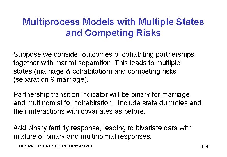
Multiprocess Models with Multiple States and Competing Risks Suppose we consider outcomes of cohabiting partnerships together with marital separation. This leads to multiple states (marriage & cohabitation) and competing risks (separation & marriage). Partnership transition indicator will be binary for marriage and multinomial for cohabitation. Include state dummies and their interactions with covariates as before. Add binary fertility response, leading to bivariate data with mixture of binary and multinomial responses. Multilevel Discrete-Time Event History Analysis 124

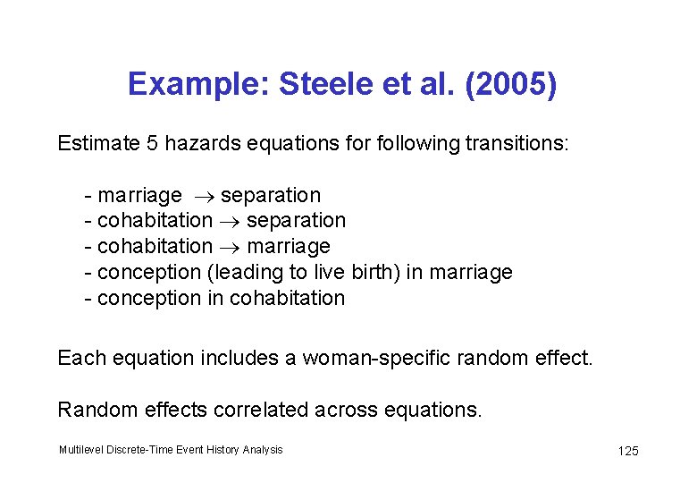
Example: Steele et al. (2005) Estimate 5 hazards equations for following transitions: - marriage separation - cohabitation marriage - conception (leading to live birth) in marriage - conception in cohabitation Each equation includes a woman-specific random effect. Random effects correlated across equations. Multilevel Discrete-Time Event History Analysis 125

Random Effects Covariance Matrix: Partnership Transitions Multilevel Discrete-Time Event History Analysis 126

Random Effects Covariance Matrix: Fertility Multilevel Discrete-Time Event History Analysis 127

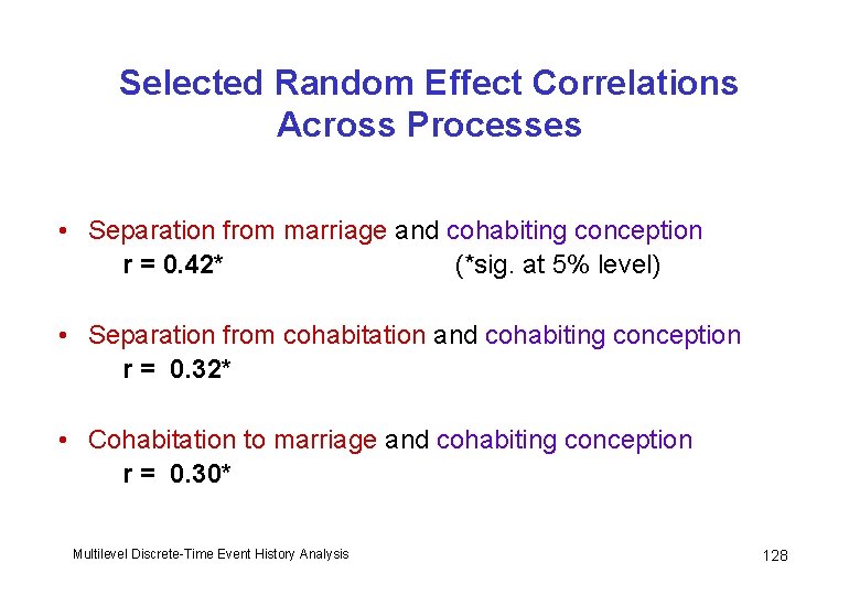
Selected Random Effect Correlations Across Processes • Separation from marriage and cohabiting conception r = 0. 42* (*sig. at 5% level) • Separation from cohabitation and cohabiting conception r = 0. 32* • Cohabitation to marriage and cohabiting conception r = 0. 30* Multilevel Discrete-Time Event History Analysis 128

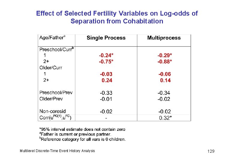
Effect of Selected Fertility Variables on Log-odds of Separation from Cohabitation Multilevel Discrete-Time Event History Analysis 129

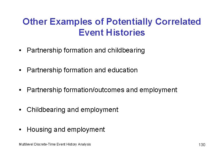
Other Examples of Potentially Correlated Event Histories • Partnership formation and childbearing • Partnership formation and education • Partnership formation/outcomes and employment • Childbearing and employment • Housing and employment Multilevel Discrete-Time Event History Analysis 130

Bibliography: Modelling the Time to a Single Event Allison, P. D. (1982) “Discrete-time methods for the analysis of event history data. ” In Sociological Methodology (Ed. S. Leinhardt). San Francisco: Jossey-Bass. Singer, J. D. and Willet, J. B. (1993) “It’s about time: Using discrete-time survival analysis to study duration and the timing of events. ” Journal of Educational Statistics, 18: 155 -195. Multilevel Discrete-Time Event History Analysis 131

Bibliography: Models for Recurrent Events and Unobserved Heterogeneity Davis, R. B. , Elias, P. and Penn, R. (1992) “The relationship between a husband’s unemployment and a wife’s participation in the labour-force. ” Oxford Bulletin of Economics and Statistics, 54: 145 -71. Kravdal, Ø. (2001) “The high fertility of college educated women in Norway: An artefact of the separate modelling of each parity transition. ” Demographic Research, 5, Article 6. Multilevel Discrete-Time Event History Analysis 132

Bibliography: Modelling Transitions Between Multiple States Enberg, J. , Gottschalk, P. and Wolf, D. (1990) “A random-effects logit model of work-welfare transitions. ” Journal of Econometrics, 43: 63 -75. Goldstein, H. , Pan, H. and Bynner, J. (2004) “A flexible procedure for analysing longitudinal event histories using a multilevel model. ” Understanding Statistics, 3: 85 -99. Steele, F. , Goldstein, H. and Browne, W. (2004) “A general multistate competing risks model for event history data, with an application to a study of contraceptive use dynamics. ” Journal of Statistical Modelling, 4: 145 -159. Steele, F. , Kallis, C. , Goldstein, H. and Joshi, H. (2005) “The relationship between childbearing and transitions from marriage and cohabitation in Britain. ” Demography, 42: 647 -673. Multilevel Discrete-Time Event History Analysis 133

Bibliography: Modelling Competing Risks Enberg, J. , Gottschalk, P. and Wolf, D. (1990) “A random-effects logit model of work-welfare transitions. ” Journal of Econometrics, 43: 63 -75. Hill, D. H. , Axinn, W. G. and Thornton, A. (1993) “Competing hazards with shared unmeasured risk factors. ” Sociological Methodology, 23: 245 -277. Steele, F. , Diamond, I. and Wang, D. (1996) “The determinants of the duration of contraceptive use in China: A multilevel multinomial discrete hazards modelling approach. ” Demography, 33: 12‑ 33. Steele, F. , Goldstein, H. and Browne, W. (2004) “A general multistate competing risks model for event history data, with an application to a study of contraceptive use dynamics. ” Journal of Statistical Modelling, 4: 145 -159. Multilevel Discrete-Time Event History Analysis 134

Bibliography: Multiprocess Models for Correlated Histories Brien, M. J. , Lillard, L. A. and Waite, L. J. (1999) “Interrelated family-building behaviors: Cohabitation, marriage, and nonmarital conception. ” Demography, 36: 535 -551. Steele, F. , Kallis, C. , Goldstein, H. and Joshi, H. (2005) “The relationship between childbearing and transitions from marriage and cohabitation in Britain. ” Demography, 42: 647 -673. Upchurch, D. M. , Lillard, L. A. and Panis, C. W. A. (2002) “Nonmarital childbearing: Influences of education, marriage, and fertility. ” Demography, 39: 311 -329. Waite, L. J. and Lillard, L. A. 1991. “Children and marital disruption. ” American Journal of Sociology, 96: 930 -53. Multilevel Discrete-Time Event History Analysis 135