DiscreteTime Models Lecture 1 When To Use DiscreteTime

Discrete-Time Models Lecture 1

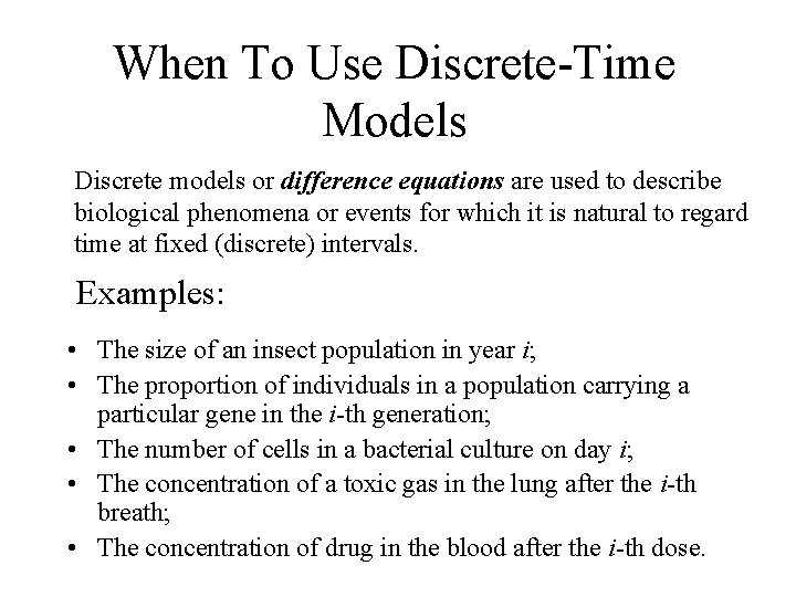
When To Use Discrete-Time Models Discrete models or difference equations are used to describe biological phenomena or events for which it is natural to regard time at fixed (discrete) intervals. Examples: • The size of an insect population in year i; • The proportion of individuals in a population carrying a particular gene in the i-th generation; • The number of cells in a bacterial culture on day i; • The concentration of a toxic gas in the lung after the i-th breath; • The concentration of drug in the blood after the i-th dose.

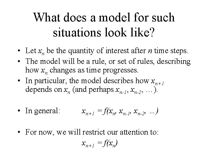
What does a model for such situations look like? • Let xn be the quantity of interest after n time steps. • The model will be a rule, or set of rules, describing how xn changes as time progresses. • In particular, the model describes how xn+1 depends on xn (and perhaps xn-1, xn-2, …). • In general: xn+1 = f(xn, xn-1, xn-2, …) • For now, we will restrict our attention to: xn+1 = f(xn)

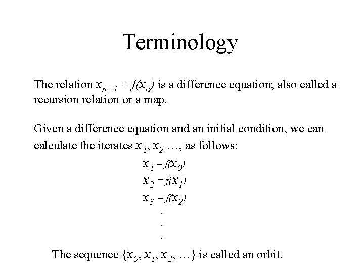
Terminology The relation xn+1 = f(xn) is a difference equation; also called a recursion relation or a map. Given a difference equation and an initial condition, we can calculate the iterates x 1, x 2 …, as follows: x 1 = f(x 0) x 2 = f(x 1) x 3 = f(x 2). . . The sequence {x 0, x 1, x 2, …} is called an orbit.

Question • Given the difference equation xn+1 = f(xn) can we make predictions about the characteristics of its orbits?

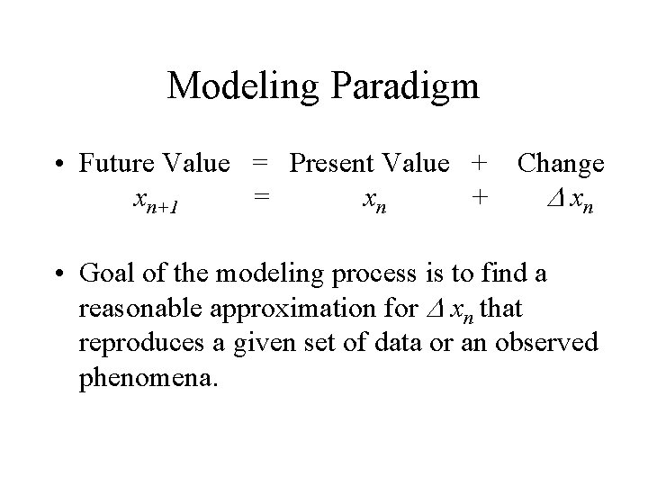
Modeling Paradigm • Future Value = Present Value + Change xn+1 = xn + D xn • Goal of the modeling process is to find a reasonable approximation for D xn that reproduces a given set of data or an observed phenomena.

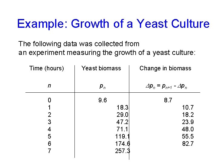
Example: Growth of a Yeast Culture The following data was collected from an experiment measuring the growth of a yeast culture: Time (hours) Yeast biomass Change in biomass n pn Dpn = pn+1 - Dpn 0 1 2 3 4 5 6 7 9. 6 8. 7 18. 3 29. 0 47. 2 71. 1 119. 1 174. 6 257. 3 10. 7 18. 2 23. 9 48. 0 55. 5 82. 7

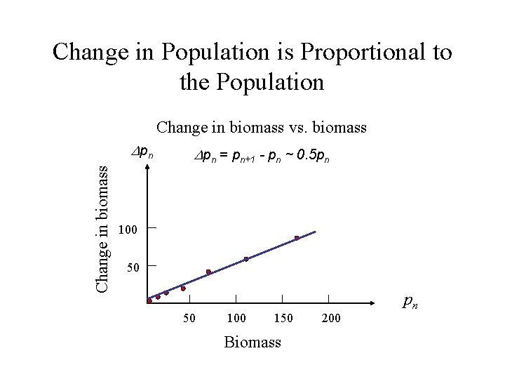
Change in Population is Proportional to the Population Change in biomass vs. biomass Change in biomass D pn Dpn = pn+1 - pn ~ 0. 5 pn 100 50 50 100 150 Biomass 200 pn

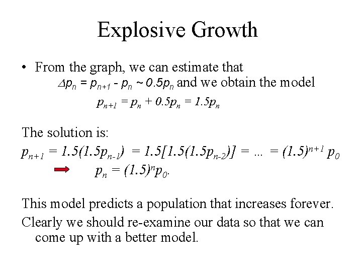
Explosive Growth • From the graph, we can estimate that Dpn = pn+1 - pn ~ 0. 5 pn and we obtain the model pn+1 = pn + 0. 5 pn = 1. 5 pn The solution is: pn+1 = 1. 5(1. 5 pn-1) = 1. 5[1. 5(1. 5 pn-2)] = … = (1. 5)n+1 p 0 pn = (1. 5)np 0. This model predicts a population that increases forever. Clearly we should re-examine our data so that we can come up with a better model.

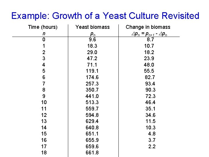
Example: Growth of a Yeast Culture Revisited Time (hours) n 0 1 2 3 4 5 6 7 8 9 10 11 12 13 14 15 16 17 18 Yeast biomass pn 9. 6 18. 3 29. 0 47. 2 71. 1 119. 1 174. 6 257. 3 350. 7 441. 0 513. 3 559. 7 594. 8 629. 4 640. 8 651. 1 655. 9 659. 6 661. 8 Change in biomass Dpn = pn+1 - Dpn 8. 7 10. 7 18. 2 23. 9 48. 0 55. 5 82. 7 93. 4 90. 3 72. 3 46. 4 35. 1 34. 6 11. 5 10. 3 4. 8 3. 7 2. 2

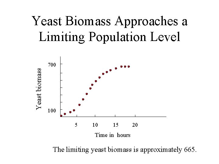
Yeast Biomass Approaches a Limiting Population Level Yeast biomass 700 100 5 10 15 20 Time in hours The limiting yeast biomass is approximately 665.

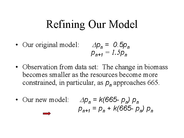
Refining Our Model • Our original model: Dpn = 0. 5 pn pn+1 = 1. 5 pn • Observation from data set: The change in biomass becomes smaller as the resources become more constrained, in particular, as pn approaches 665. • Our new model: Dpn = k(665 - pn) pn pn+1 = pn + k(665 - pn) pn

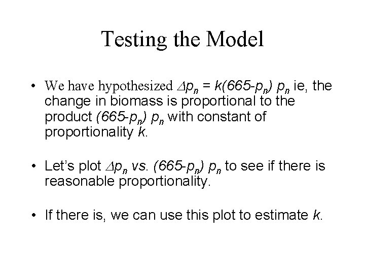
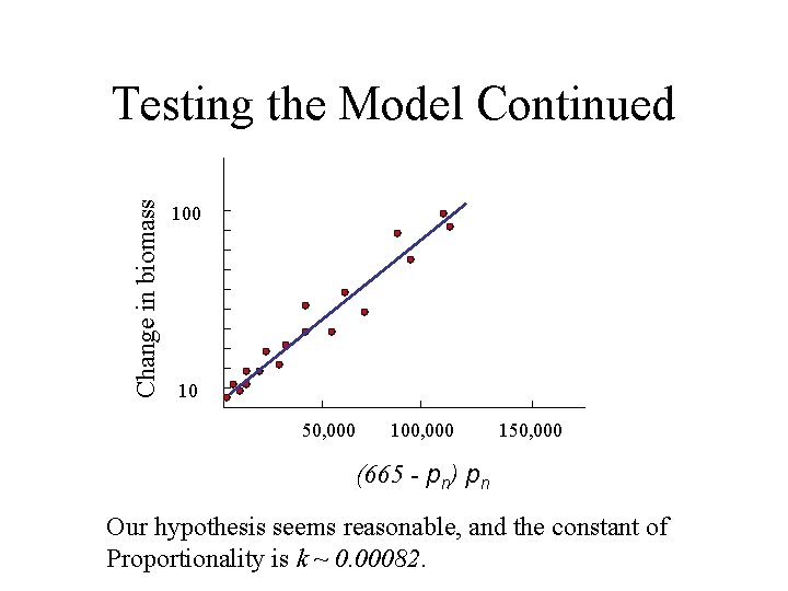
Testing the Model • We have hypothesized Dpn = k(665 -pn) pn ie, the change in biomass is proportional to the product (665 -pn) pn with constant of proportionality k. • Let’s plot Dpn vs. (665 -pn) pn to see if there is reasonable proportionality. • If there is, we can use this plot to estimate k.

Change in biomass Testing the Model Continued 100 10 50, 000 100, 000 150, 000 (665 - pn) pn Our hypothesis seems reasonable, and the constant of Proportionality is k ~ 0. 00082.

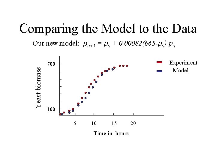
Comparing the Model to the Data Our new model: pn+1 = pn + 0. 00082(665 -pn) pn Experiment Model Yeast biomass 700 100 5 10 15 Time in hours 20

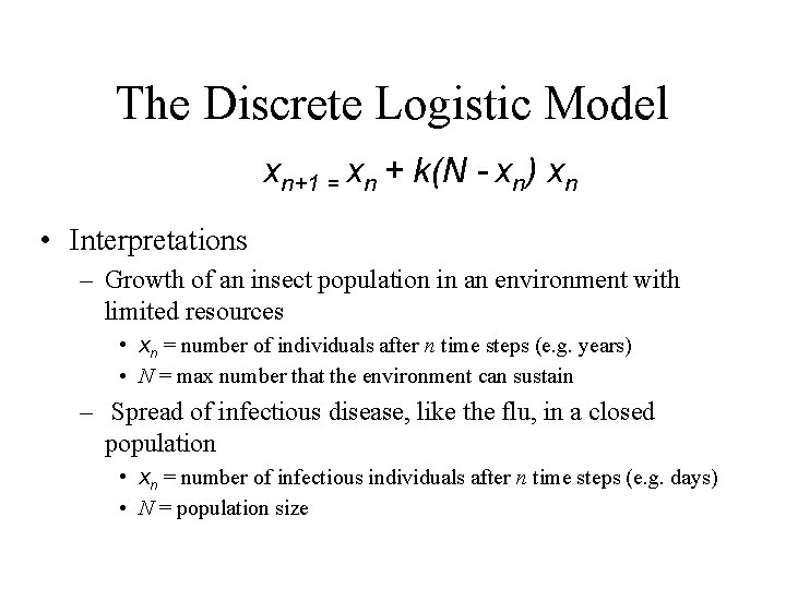
The Discrete Logistic Model xn+1 = xn + k(N - xn) xn • Interpretations – Growth of an insect population in an environment with limited resources • xn = number of individuals after n time steps (e. g. years) • N = max number that the environment can sustain – Spread of infectious disease, like the flu, in a closed population • xn = number of infectious individuals after n time steps (e. g. days) • N = population size