Multilevel Models 2 Sociology 229 Advanced Regression Copyright

Multilevel Models 2 Sociology 229: Advanced Regression Copyright © 2010 by Evan Schofer Do not copy or distribute without permission

Announcements • Assignment 5 Handed out

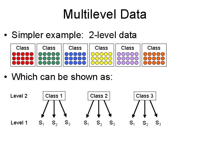
Multilevel Data • Simpler example: 2 -level data Class Class • Which can be shown as: Class 1 Level 2 Level 1 S 2 Class 2 S 3 S 1 S 2 Class 3 S 1 S 2 S 3

Review: Multilevel Data: Problems • Issue: Multilevel data often results in violation of OLS regression assumption • OLS requires an independent random sample… • Students from the same class (or school) are not independent… and may have correlated error – Models tend to underestimate standard errors • This leads to false rejection of H 0. – When is multilevel data NOT a problem? • Answer: If you can successfully control for potential sources of correlated error

Multilevel Data: Research Purposes • Multilevel models are more than a “fix” for problems of OLS. Uses: – Raudenbush & Bryk 2002: 8 -9 – 1. Improved estimation of individual effects • Take advantage of pooling; between/within variance – 2. Modeling cross-level effects • Separating effects of individual-level variables from social context – 3. Partitioning variance-covariance components • An important descriptive issue: At what level is most of the variance?

Review: Multilevel Data • OLS: underestimated SEs • Robust Cluster SEs • A correction for OLS • Aggregation: Focus on “between group” effects • Loss of sample size • Watch for ecological fallacy • Fixed effects: “within group” effects • Random effects: Hybrid “within” & “between” • Requires strong assumption that Xs uncorrelated with error.

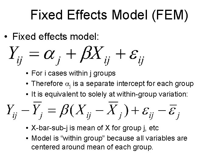
Fixed Effects Model (FEM) • Fixed effects model: • For i cases within j groups • Therefore aj is a separate intercept for each group • It is equivalent to solely at within-group variation: • X-bar-sub-j is mean of X for group j, etc • Model is “within group” because all variables are centered around mean of each group.

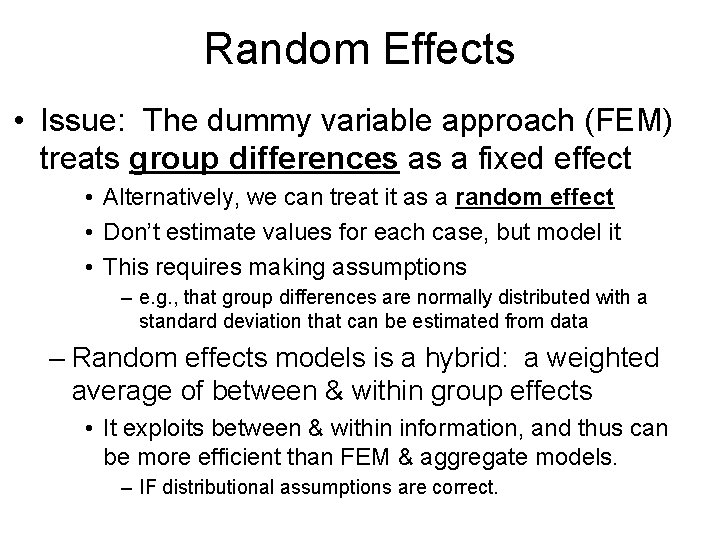
Random Effects • Issue: The dummy variable approach (FEM) treats group differences as a fixed effect • Alternatively, we can treat it as a random effect • Don’t estimate values for each case, but model it • This requires making assumptions – e. g. , that group differences are normally distributed with a standard deviation that can be estimated from data – Random effects models is a hybrid: a weighted average of between & within group effects • It exploits between & within information, and thus can be more efficient than FEM & aggregate models. – IF distributional assumptions are correct.

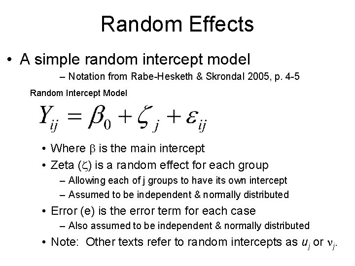
Random Effects • A simple random intercept model – Notation from Rabe-Hesketh & Skrondal 2005, p. 4 -5 Random Intercept Model • Where b is the main intercept • Zeta (z) is a random effect for each group – Allowing each of j groups to have its own intercept – Assumed to be independent & normally distributed • Error (e) is the error term for each case – Also assumed to be independent & normally distributed • Note: Other texts refer to random intercepts as uj or nj.

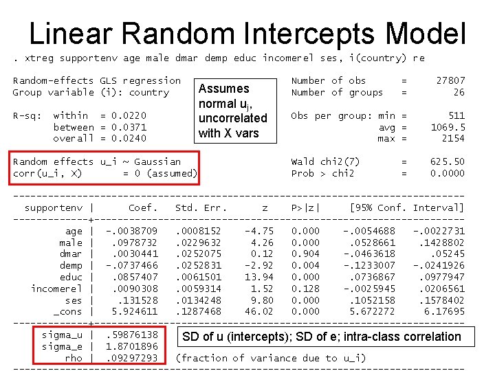
Linear Random Intercepts Model. xtreg supportenv age male dmar demp educ incomerel ses, i(country) re Random-effects GLS regression Group variable (i): country R-sq: within = 0. 0220 between = 0. 0371 overall = 0. 0240 Random effects u_i ~ Gaussian corr(u_i, X) = 0 (assumed) Assumes normal uj, uncorrelated with X vars Number of obs Number of groups = = 27807 26 Obs per group: min = avg = max = 511 1069. 5 2154 Wald chi 2(7) Prob > chi 2 625. 50 0. 0000 = = ---------------------------------------supportenv | Coef. Std. Err. z P>|z| [95% Conf. Interval] -------+--------------------------------age | -. 0038709. 0008152 -4. 75 0. 000 -. 0054688 -. 0022731 male |. 0978732. 0229632 4. 26 0. 000. 0528661. 1428802 dmar |. 0030441. 0252075 0. 12 0. 904 -. 0463618. 05245 demp | -. 0737466. 0252831 -2. 92 0. 004 -. 1233007 -. 0241926 educ |. 0857407. 0061501 13. 94 0. 000. 0736867. 0977947 incomerel |. 0090308. 0059314 1. 52 0. 128 -. 0025945. 0206561 ses |. 131528. 0134248 9. 80 0. 000. 1052158. 1578402 _cons | 5. 924611. 1287468 46. 02 0. 000 5. 672272 6. 17695 -------+--------------------------------sigma_u |. 59876138 SD of u (intercepts); SD of e; intra-class correlation sigma_e | 1. 8701896 rho |. 09297293 (fraction of variance due to u_i)

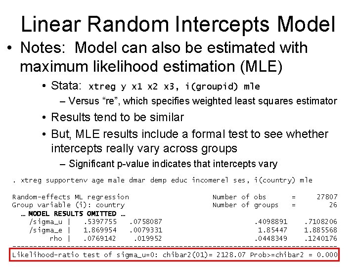
Linear Random Intercepts Model • Notes: Model can also be estimated with maximum likelihood estimation (MLE) • Stata: xtreg y x 1 x 2 x 3, i(groupid) mle – Versus “re”, which specifies weighted least squares estimator • Results tend to be similar • But, MLE results include a formal test to see whether intercepts really vary across groups – Significant p-value indicates that intercepts vary. xtreg supportenv age male dmar demp educ incomerel ses, i(country) mle Random-effects ML regression Number of obs = 27807 Group variable (i): country Number of groups = 26 … MODEL RESULTS OMITTED … /sigma_u |. 5397755. 0758087. 4098891. 7108206 /sigma_e | 1. 869954. 0079331 1. 85447 1. 885568 rho |. 0769142. 019952. 0448349. 1240176 ---------------------------------------Likelihood-ratio test of sigma_u=0: chibar 2(01)= 2128. 07 Prob>=chibar 2 = 0. 000

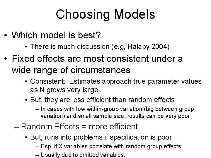
Choosing Models • Which model is best? • There is much discussion (e. g, Halaby 2004) • Fixed effects are most consistent under a wide range of circumstances • Consistent: Estimates approach true parameter values as N grows very large • But, they are less efficient than random effects – In cases with low within-group variation (big between group variation) and small sample size, results can be very poor – Random Effects = more efficient • But, runs into problems if specification is poor – Esp. if X variables correlate with random group effects – Usually due to omitted variables.

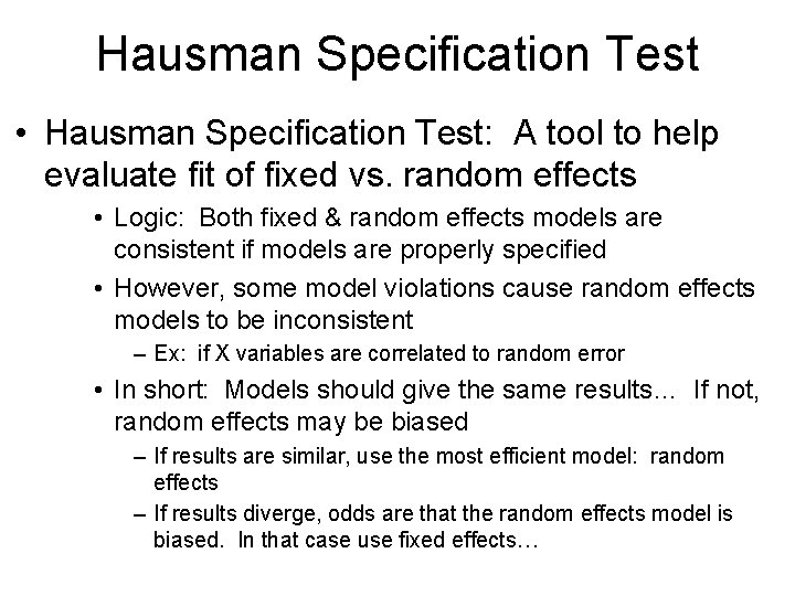
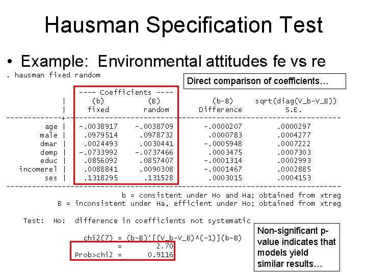
Hausman Specification Test • Hausman Specification Test: A tool to help evaluate fit of fixed vs. random effects • Logic: Both fixed & random effects models are consistent if models are properly specified • However, some model violations cause random effects models to be inconsistent – Ex: if X variables are correlated to random error • In short: Models should give the same results… If not, random effects may be biased – If results are similar, use the most efficient model: random effects – If results diverge, odds are that the random effects model is biased. In that case use fixed effects…

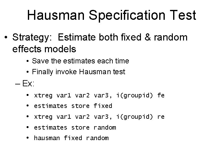
Hausman Specification Test • Strategy: Estimate both fixed & random effects models • Save the estimates each time • Finally invoke Hausman test – Ex: • • • xtreg var 1 var 2 var 3, i(groupid) fe estimates store fixed xtreg var 1 var 2 var 3, i(groupid) re estimates store random hausman fixed random

Hausman Specification Test • Example: Environmental attitudes fe vs re. hausman fixed random Direct comparison of coefficients… ---- Coefficients ---| (b) (B) (b-B) sqrt(diag(V_b-V_B)) | fixed random Difference S. E. -------+--------------------------------age | -. 0038917 -. 0038709 -. 0000207. 0000297 male |. 0979514. 0978732. 0000783. 0004277 dmar |. 0024493. 0030441 -. 0005948. 0007222 demp | -. 0733992 -. 0737466. 0003475. 0007303 educ |. 0856092. 0857407 -. 0001314. 0002993 incomerel |. 0088841. 0090308 -. 0001467. 0002885 ses |. 1318295. 131528. 0003015. 0004153 ---------------------------------------b = consistent under Ho and Ha; obtained from xtreg B = inconsistent under Ha, efficient under Ho; obtained from xtreg Test: Ho: difference in coefficients not systematic chi 2(7) = (b-B)'[(V_b-V_B)^(-1)](b-B) = 2. 70 Prob>chi 2 = 0. 9116 Non-significant pvalue indicates that models yield similar results…

Within & Between Effects • Issue: What is the relationship between within -group effects and between-group effects? • FEM models within-group variation • BEM models between group variation (aggregate) – Usually they are similar • Ex: Student skills & test performance • Within any classroom, skilled students do best on tests • Between classrooms, classes with more skilled students have higher mean test scores – BUT…

Within & Between Effects • But: Between and within effects can differ! • Ex: Effects of wealth on attitudes toward welfare • At the country level (between groups): – Wealthier countries (high aggregate mean) tend to have prowelfare attitudes (ex: Scandinavia) • At the individual level (within group) – Wealthier people are conservative, don’t support welfare • Result: Wealth has opposite between vs within effects! – Watch out for ecological fallacy!!! – Issue: Such dynamics often result from omitted level-1 variables (omitted variable bias) • Ex: If we control for individual “political conservatism”, effects may be consistent at both levels…

Within & Between Effects / Centering • Multilevel models & “centering” variables • Grand mean centering: computing variables as deviations from overall mean • Often done to X variables • Has effect that baseline constant in model reflects mean of all cases – Useful for interpretation • Group mean centering: computing variables as deviation from group mean • Useful for decomposing within vs. between effects • Often in conjunction with aggregate group mean vars.

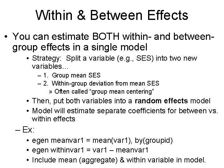
Within & Between Effects • You can estimate BOTH within- and betweengroup effects in a single model • Strategy: Split a variable (e. g. , SES) into two new variables… – 1. Group mean SES – 2. Within-group deviation from mean SES » Often called “group mean centering” • Then, put both variables into a random effects model • Model will estimate separate coefficients for between vs. within effects – Ex: • egen meanvar 1 = mean(var 1), by(groupid) • egen withinvar 1 = var 1 – meanvar 1 • Include mean (aggregate) & within variable in model.

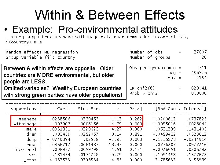
Within & Between Effects • Example: Pro-environmental attitudes. xtreg supportenv meanage withinage male dmar demp educ incomerel ses, i(country) mle Random-effects ML regression Group variable (i): country Random effects ~ Gaussian Between & withinu_i effects are opposite. Older countries are MORE environmental, but older people are LESS. Omitted variables? Wealthy European countries Log strong likelihood -56918. 299 with green =parties have older populations! Number of obs Number of groups = = 27807 26 Obs per group: min = avg = max = 511 1069. 5 2154 LR chi 2(8) Prob > chi 2 620. 41 0. 0000 = = ---------------------------------------supportenv | Coef. Std. Err. z P>|z| [95% Conf. Interval] -------+--------------------------------meanage |. 0268506. 0239453 1. 12 0. 262 -. 0200812. 0737825 withinage | -. 003903. 0008156 -4. 79 0. 000 -. 0055016 -. 0023044 male |. 0981351. 0229623 4. 27 0. 000. 0531299. 1431403 dmar |. 003459. 0252057 0. 14 0. 891 -. 0459432. 0528612 demp | -. 0740394. 02528 -2. 93 0. 003 -. 1235873 -. 0244914 educ |. 0856712. 0061483 13. 93 0. 000. 0736207. 0977216 incomerel |. 008957. 0059298 1. 51 0. 131 -. 0026651. 0205792 ses |. 131454. 0134228 9. 79 0. 000. 1051458. 1577622 _cons | 4. 687526. 9703564 4. 83 0. 000 2. 785662 6. 58939

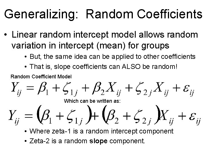
Generalizing: Random Coefficients • Linear random intercept model allows random variation in intercept (mean) for groups • But, the same idea can be applied to other coefficients • That is, slope coefficients can ALSO be random! Random Coefficient Model Which can be written as: • Where zeta-1 is a random intercept component • Zeta-2 is a random slope component.

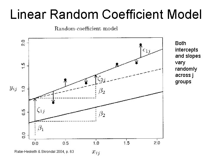
Linear Random Coefficient Model Both intercepts and slopes vary randomly across j groups Rabe-Hesketh & Skrondal 2004, p. 63

Random Coefficients Summary • Some things to remember: • Dummy variables allow fixed estimates of intercepts across groups • Interactions allow fixed estimates of slopes across groups – Random coefficients allow intercepts and/or slopes to have random variability • The model does not directly estimate those effects – Just as we don’t estimate coefficients of “e” for each case… • BUT, random components can be predicted after you run a model – Just as you can compute residuals – random error – This allows you to examine some assumptions (normality).

STATA Notes: xtreg, xtmixed • xtreg – allows estimation of between, within (fixed), and random intercept models • • xtreg y x 1 x 2 x 3, i(groupid) fe - fixed (within) model xtreg y x 1 x 2 x 3, i(groupid) be - between model xtreg y x 1 x 2 x 3, i(groupid) re - random intercept (GLS) xtreg y x 1 x 2 x 3, i(groupid) mle - random intercept (MLE) • xtmixed – allows random intercepts & slopes • “Mixed” models refer to models that have both fixed and random components • xtmixed [depvar] [fixed equation] || [random eq], options • Ex: xtmixed y x 1 x 2 x 3 || groupid: x 2 – Random intercept is assumed. Random coef for X 2 specified.

STATA Notes: xtreg, xtmixed • Random intercepts • xtreg y x 1 x 2 x 3, i(groupid) mle – Is equivalent to • xtmixed y x 1 x 2 x 3 || groupid: , mle • xtmixed assumes random intercept – even if no other random effects are specified after “groupid” – But, we can add random coefficients for all Xs: • xtmixed y x 1 x 2 x 3 || groupid: x 1 x 2 x 3 , mle cov(unstr) – Useful to add: “cov(unstructured)” • Stata default treats random terms (intercept, slope) as totally uncorrelated… not always reasonable • “cov(unstr) relaxes constraints regarding covariance among random effects (See Rabe-Hesketh & Skrondal).

STATA Notes: GLLAMM • Note: xtmixed can do a lot… but GLLAMM can do even more! • “General linear & latent mixed models” • Must be downloaded into stata. Type “search gllamm” and follow instructions to install… – GLLAMM can do a wide range of mixed & latentvariable models • Multilevel models; Some kinds of latent class models; Confirmatory factor analysis; Some kinds of Structural Equation Models with latent variables… and others… • Documentation available via Stata help – And, in the Rabe-Hesketh & Skrondal text.

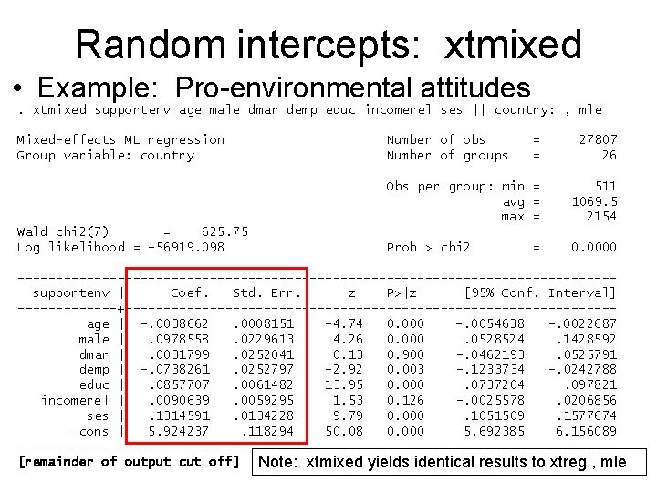
Random intercepts: xtmixed • Example: Pro-environmental attitudes. xtmixed supportenv age male dmar demp educ incomerel ses || country: , mle Mixed-effects ML regression Group variable: country Wald chi 2(7) = 625. 75 Log likelihood = -56919. 098 Number of obs Number of groups = = 27807 26 Obs per group: min = avg = max = 511 1069. 5 2154 Prob > chi 2 0. 0000 = ---------------------------------------supportenv | Coef. Std. Err. z P>|z| [95% Conf. Interval] -------+--------------------------------age | -. 0038662. 0008151 -4. 74 0. 000 -. 0054638 -. 0022687 male |. 0978558. 0229613 4. 26 0. 000. 0528524. 1428592 dmar |. 0031799. 0252041 0. 13 0. 900 -. 0462193. 0525791 demp | -. 0738261. 0252797 -2. 92 0. 003 -. 1233734 -. 0242788 educ |. 0857707. 0061482 13. 95 0. 000. 0737204. 097821 incomerel |. 0090639. 0059295 1. 53 0. 126 -. 0025578. 0206856 ses |. 1314591. 0134228 9. 79 0. 000. 1051509. 1577674 _cons | 5. 924237. 118294 50. 08 0. 000 5. 692385 6. 156089 ---------------------------------------[remainder of output cut off] Note: xtmixed yields identical results to xtreg , mle

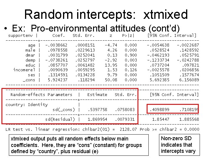
Random intercepts: xtmixed • Ex: Pro-environmental attitudes (cont’d) supportenv | Coef. Std. Err. z P>|z| [95% Conf. Interval] -------+--------------------------------age | -. 0038662. 0008151 -4. 74 0. 000 -. 0054638 -. 0022687 male |. 0978558. 0229613 4. 26 0. 000. 0528524. 1428592 dmar |. 0031799. 0252041 0. 13 0. 900 -. 0462193. 0525791 demp | -. 0738261. 0252797 -2. 92 0. 003 -. 1233734 -. 0242788 educ |. 0857707. 0061482 13. 95 0. 000. 0737204. 097821 incomerel |. 0090639. 0059295 1. 53 0. 126 -. 0025578. 0206856 ses |. 1314591. 0134228 9. 79 0. 000. 1051509. 1577674 _cons | 5. 924237. 118294 50. 08 0. 000 5. 692385 6. 156089 -----------------------------------------------------------------------------Random-effects Parameters | Estimate Std. Err. [95% Conf. Interval] ---------------+------------------------country: Identity | sd(_cons) |. 5397758. 0758083. 4098899. 7108199 ---------------+------------------------sd(Residual) | 1. 869954. 0079331 1. 85447 1. 885568 ---------------------------------------LR test vs. linear regression: chibar 2(01) = 2128. 07 Prob >= chibar 2 = 0. 0000 xtmixed output puts all random effects below main coefficients. Here, they are “cons” (constant) for groups defined by “country”, plus residual (e) Non-zero SD indicates that intercepts vary

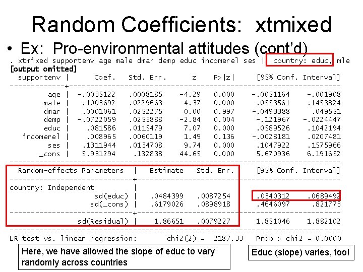
Random Coefficients: xtmixed • Ex: Pro-environmental attitudes (cont’d). xtmixed supportenv age male dmar demp educ incomerel ses || country: educ, mle [output omitted] supportenv | Coef. Std. Err. z P>|z| [95% Conf. Interval] -------+--------------------------------age | -. 0035122. 0008185 -4. 29 0. 000 -. 0051164 -. 001908 male |. 1003692. 0229663 4. 37 0. 000. 0553561. 1453824 dmar |. 0001061. 0252275 0. 00 0. 997 -. 0493388. 049551 demp | -. 0722059. 0253888 -2. 84 0. 004 -. 121967 -. 0224447 educ |. 081586. 0115479 7. 07 0. 000. 0589526. 1042194 incomerel |. 008965. 0060119 1. 49 0. 136 -. 0028181. 0207481 ses |. 1311944. 0134708 9. 74 0. 000. 1047922. 1575966 _cons | 5. 931294. 132838 44. 65 0. 000 5. 670936 6. 191652 ---------------------------------------Random-effects Parameters | Estimate Std. Err. [95% Conf. Interval] ---------------+------------------------country: Independent | sd(educ) |. 0484399. 0087254. 0340312. 0689492 sd(_cons) |. 6179026. 0898918. 4646097. 821773 ---------------+------------------------sd(Residual) | 1. 86651. 0079227 1. 851046 1. 882102 ---------------------------------------LR test vs. linear regression: chi 2(2) = 2187. 33 Prob > chi 2 = 0. 0000 Here, we have allowed the slope of educ to vary randomly across countries Educ (slope) varies, too!

Random Coefficients: xtmixed • What if the random intercept or slope coefficients aren’t significantly different from zero? • Answer: that means there isn’t much random variability in the slope/intercept • Conclusion: You don’t need to specify that random parameter – Also: Models include a LRtest to compare with a simple OLS model (no random effects) • If models don’t differ (Chi-square is not significant) stick with a simpler model.

Random Coefficients: xtmixed • What are random coefficients doing? • Let’s look at results from a simplified model – Only random slope & intercept for education Model fits a different slope & intercept for each group!

Random Coefficients • Why bother with random coefficients? – 1. A solution for clustering (non-independence) – Usually people just use random intercepts, but slopes may be an issue also – 2. You can create a better-fitting model – If slopes & intercepts vary, a random coefficient model may fit better – Assuming distributional assumptions are met – Model fit compared to OLS can be tested…. – 3. Better predictions – Attention to group-specific random effects can yield better predictions (e. g. , slopes) for each group » Rather than just looking at “average” slope for all groups.

Random Coefficients • 4. Multilevel models explicitly put attention on levels of causality • Higher level / “contextual” effects versus individual / unit -level effects • A technology for separating out between/within • NOTE: this can be done w/out random effects – But it goes hand-in-hand with clustered data… • Note: Be sure you have enough level-2 units! – Ex: Models of individual environmental attitudes • Adding level-2 effects: Democracy, GDP, etc. – Ex: Classrooms • Is it student SES, or “contextual” class/school SES?

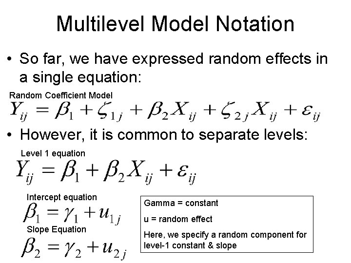
Multilevel Model Notation • So far, we have expressed random effects in a single equation: Random Coefficient Model • However, it is common to separate levels: Level 1 equation Intercept equation Gamma = constant u = random effect Slope Equation Here, we specify a random component for level-1 constant & slope

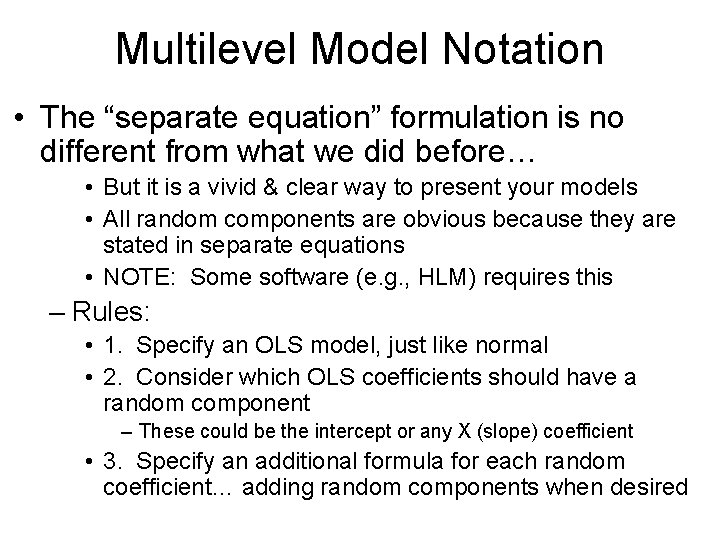
Multilevel Model Notation • The “separate equation” formulation is no different from what we did before… • But it is a vivid & clear way to present your models • All random components are obvious because they are stated in separate equations • NOTE: Some software (e. g. , HLM) requires this – Rules: • 1. Specify an OLS model, just like normal • 2. Consider which OLS coefficients should have a random component – These could be the intercept or any X (slope) coefficient • 3. Specify an additional formula for each random coefficient… adding random components when desired

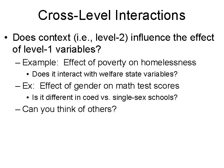
Cross-Level Interactions • Does context (i. e. , level-2) influence the effect of level-1 variables? – Example: Effect of poverty on homelessness • Does it interact with welfare state variables? – Ex: Effect of gender on math test scores • Is it different in coed vs. single-sex schools? – Can you think of others?

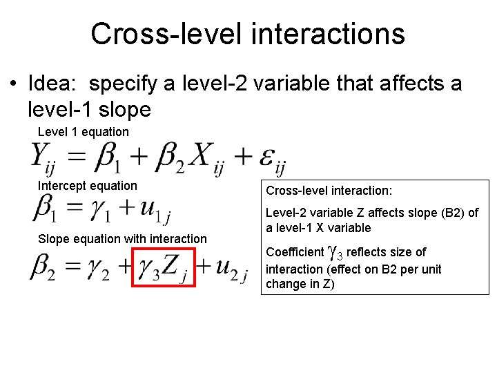
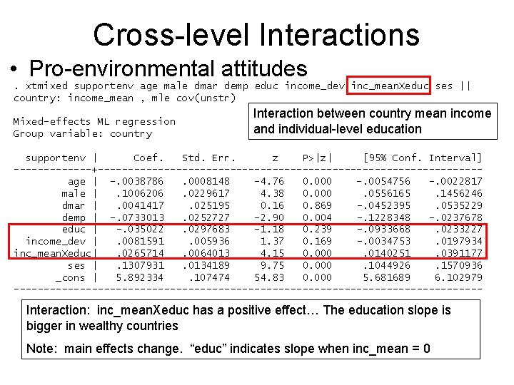
Cross-level interactions • Idea: specify a level-2 variable that affects a level-1 slope Level 1 equation Intercept equation Slope equation with interaction Cross-level interaction: Level-2 variable Z affects slope (B 2) of a level-1 X variable g Coefficient 3 reflects size of interaction (effect on B 2 per unit change in Z)

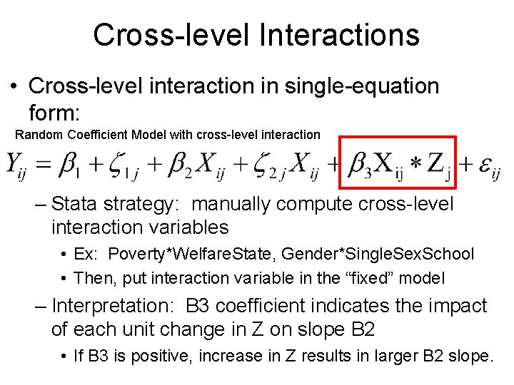
Cross-level Interactions • Cross-level interaction in single-equation form: Random Coefficient Model with cross-level interaction – Stata strategy: manually compute cross-level interaction variables • Ex: Poverty*Welfare. State, Gender*Single. Sex. School • Then, put interaction variable in the “fixed” model – Interpretation: B 3 coefficient indicates the impact of each unit change in Z on slope B 2 • If B 3 is positive, increase in Z results in larger B 2 slope.

Cross-level Interactions • Pro-environmental attitudes. xtmixed supportenv age male dmar demp educ income_dev inc_mean. Xeduc ses || country: income_mean , mle cov(unstr) Mixed-effects ML regression Group variable: country Interaction between country mean income Number of obs = 27807 and individual-level education Number of groups = 26 supportenv | Coef. Std. Err. z P>|z| [95% Conf. Interval] -------+--------------------------------age | -. 0038786. 0008148 -4. 76 0. 000 -. 0054756 -. 0022817 male |. 1006206. 0229617 4. 38 0. 000. 0556165. 1456246 dmar |. 0041417. 025195 0. 16 0. 869 -. 0452395. 0535229 demp | -. 0733013. 0252727 -2. 90 0. 004 -. 1228348 -. 0237678 educ | -. 035022. 0297683 -1. 18 0. 239 -. 0933668. 0233227 income_dev |. 0081591. 005936 1. 37 0. 169 -. 0034753. 0197934 inc_mean. Xeduc|. 0265714. 0064013 4. 15 0. 000. 0140251. 0391177 ses |. 1307931. 0134189 9. 75 0. 000. 1044926. 1570936 _cons | 5. 892334. 107474 54. 83 0. 000 5. 681689 6. 102979 --------------------------------------- Interaction: inc_mean. Xeduc has a positive effect… The education slope is bigger in wealthy countries Note: main effects change. “educ” indicates slope when inc_mean = 0

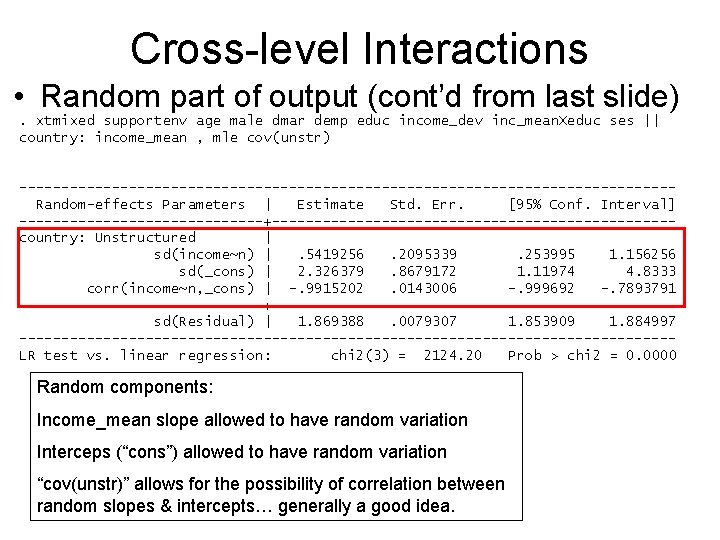
Cross-level Interactions • Random part of output (cont’d from last slide). xtmixed supportenv age male dmar demp educ income_dev inc_mean. Xeduc ses || country: income_mean , mle cov(unstr) ---------------------------------------Random-effects Parameters | Estimate Std. Err. [95% Conf. Interval] ---------------+------------------------country: Unstructured | sd(income~n) |. 5419256. 2095339. 253995 1. 156256 sd(_cons) | 2. 326379. 8679172 1. 11974 4. 8333 corr(income~n, _cons) | -. 9915202. 0143006 -. 999692 -. 7893791 ---------------+------------------------sd(Residual) | 1. 869388. 0079307 1. 853909 1. 884997 ---------------------------------------LR test vs. linear regression: chi 2(3) = 2124. 20 Prob > chi 2 = 0. 0000 Random components: Income_mean slope allowed to have random variation Interceps (“cons”) allowed to have random variation “cov(unstr)” allows for the possibility of correlation between random slopes & intercepts… generally a good idea.

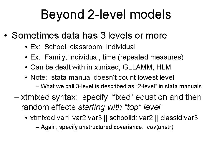
Beyond 2 -level models • Sometimes data has 3 levels or more • • Ex: School, classroom, individual Ex: Family, individual, time (repeated measures) Can be dealt with in xtmixed, GLLAMM, HLM Note: stata manual doesn’t count lowest level – What we call 3 -level is described as “ 2 -level” in stata manuals – xtmixed syntax: specify “fixed” equation and then random effects starting with “top” level • xtmixed var 1 var 2 var 3 || schoolid: var 2 || classid: var 3 – Again, specify unstructured covariance: cov(unstr)

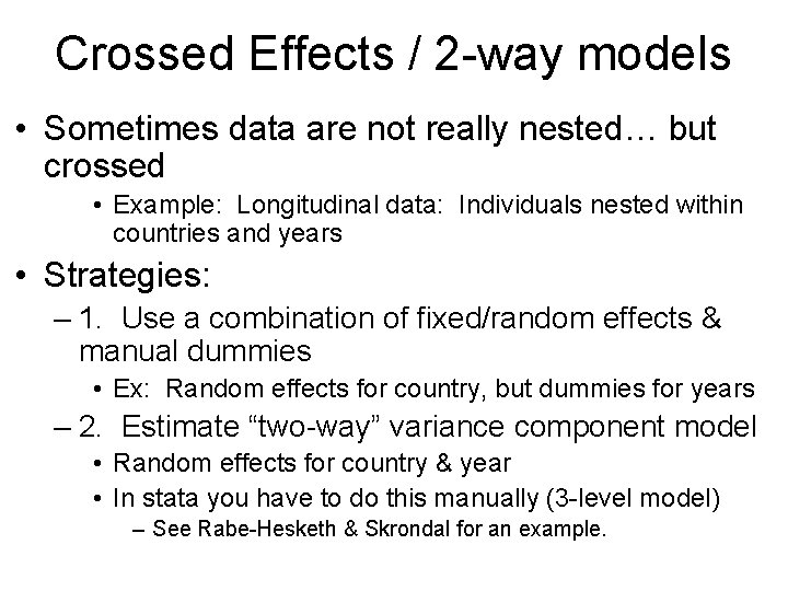
Crossed Effects / 2 -way models • Sometimes data are not really nested… but crossed • Example: Longitudinal data: Individuals nested within countries and years • Strategies: – 1. Use a combination of fixed/random effects & manual dummies • Ex: Random effects for country, but dummies for years – 2. Estimate “two-way” variance component model • Random effects for country & year • In stata you have to do this manually (3 -level model) – See Rabe-Hesketh & Skrondal for an example.

Advice about building models • Raudenbush & Bryk 2002 – Start building the level 1 model first – Then build level 2 model • Keeping a close eye on level 2 N.

Beyond Linear Models • Stata can specify multilevel models for dichotomous & count variables – Random intercept models • • xtlogit – logistic regression – dichotomous xtpois – poisson regression – counts xtnbreg – negative binomial – counts xtgee – any family, link… w/random intercept – Random intercept & coefficient models – Plus, allows more than 2 levels… • xtmelogit – mixed logit model • xtmepoisson – mixed poisson model

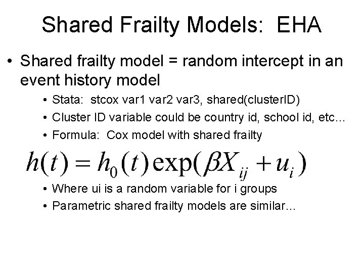
Shared Frailty Models: EHA • Shared frailty model = random intercept in an event history model • Stata: stcox var 1 var 2 var 3, shared(cluster. ID) • Cluster ID variable could be country id, school id, etc… • Formula: Cox model with shared frailty • Where ui is a random variable for i groups • Parametric shared frailty models are similar…

Shared Frailty Models: EHA • Shared frailty (random effects) are useful for: – 1. Clustered data • Just like prior examples – 2. Models with repeated events • Repeated events is a kind of clustering within caseid • Again, dummy variables (FEM) is a reasonable option – In stata, you’d have to enter the dummies manually • Stata: specify cluster ID and form of frailty • stcox var 1 var 2, frailty(gamma) shared(schoolid) • streg var 1 var 2, dist(e) frailty(gamma) shared(schoolid)

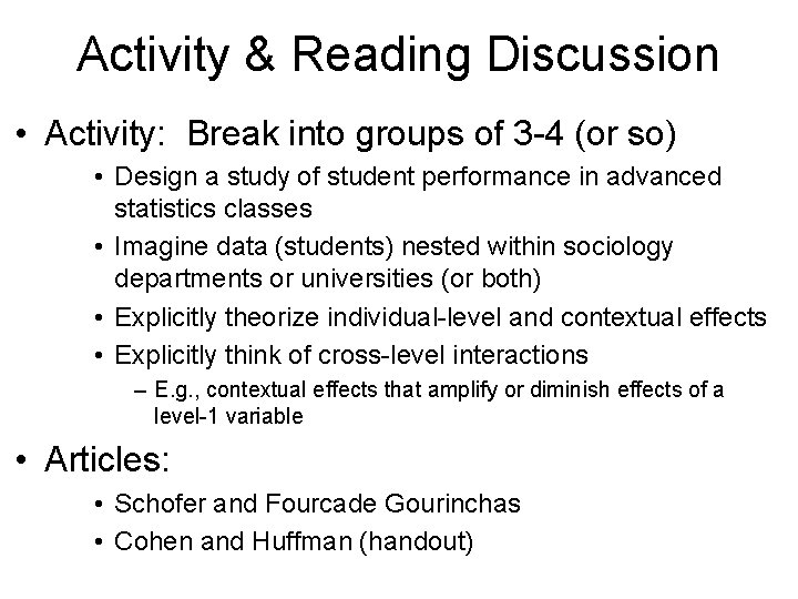
Activity & Reading Discussion • Activity: Break into groups of 3 -4 (or so) • Design a study of student performance in advanced statistics classes • Imagine data (students) nested within sociology departments or universities (or both) • Explicitly theorize individual-level and contextual effects • Explicitly think of cross-level interactions – E. g. , contextual effects that amplify or diminish effects of a level-1 variable • Articles: • Schofer and Fourcade Gourinchas • Cohen and Huffman (handout)

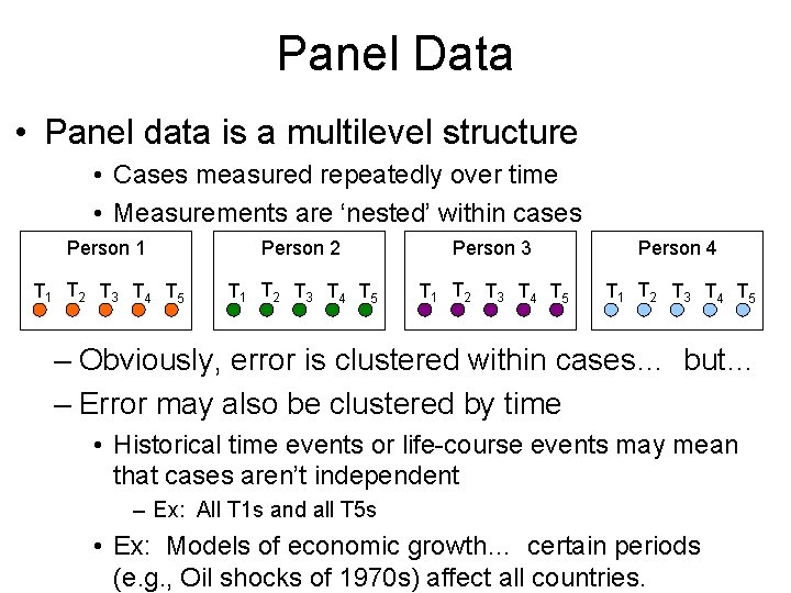
Panel Data • Panel data is a multilevel structure • Cases measured repeatedly over time • Measurements are ‘nested’ within cases Person 1 Person 2 Person 3 Person 4 T 1 T 2 T 3 T 4 T 5 – Obviously, error is clustered within cases… but… – Error may also be clustered by time • Historical time events or life-course events may mean that cases aren’t independent – Ex: All T 1 s and all T 5 s • Ex: Models of economic growth… certain periods (e. g. , Oil shocks of 1970 s) affect all countries.

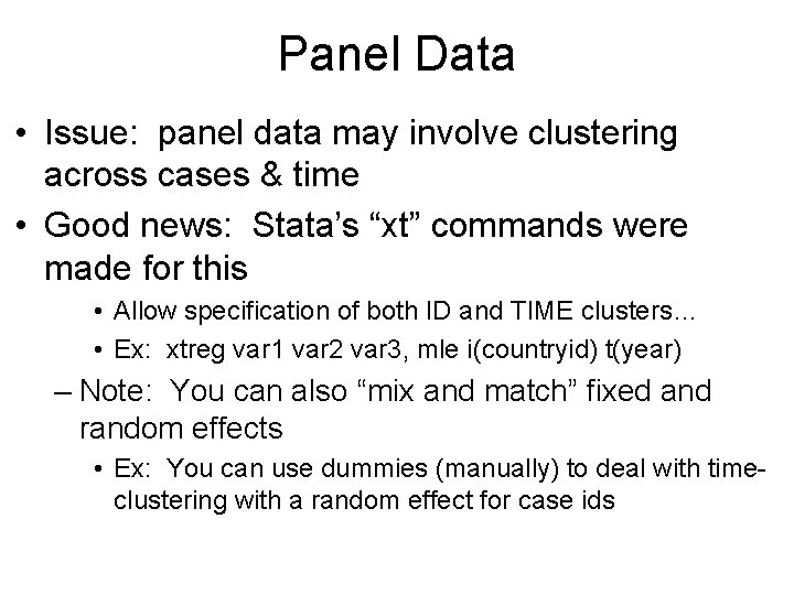
Panel Data • Issue: panel data may involve clustering across cases & time • Good news: Stata’s “xt” commands were made for this • Allow specification of both ID and TIME clusters… • Ex: xtreg var 1 var 2 var 3, mle i(countryid) t(year) – Note: You can also “mix and match” fixed and random effects • Ex: You can use dummies (manually) to deal with timeclustering with a random effect for case ids

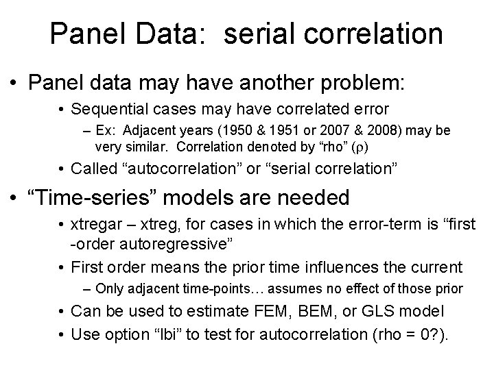
Panel Data: serial correlation • Panel data may have another problem: • Sequential cases may have correlated error – Ex: Adjacent years (1950 & 1951 or 2007 & 2008) may be very similar. Correlation denoted by “rho” (r) • Called “autocorrelation” or “serial correlation” • “Time-series” models are needed • xtregar – xtreg, for cases in which the error-term is “first -order autoregressive” • First order means the prior time influences the current – Only adjacent time-points… assumes no effect of those prior • Can be used to estimate FEM, BEM, or GLS model • Use option “lbi” to test for autocorrelation (rho = 0? ).

Panel Data: Choosing a Model • If clustering is mainly a nuisance: • Adjust SEs: vce(cluster caseid) • Or simple fixed or random effects – Choice between fixed & random • Hausman test is one way to decide • Fixed is “safer” – reviewers are less likely to complain • But, if cross-sectional variation is of interest, fixed can be a problem… – In that case, use random effects… and hope the reviewers don’t give you grief – More on panel data next week!