Operating Systems CPU Scheduling Algorithms Note Some slides

Operating Systems CPU Scheduling Algorithms Note: Some slides and/or pictures are adapted from Lecture slides / Books of • • Dr Mansoor Sarwar. Dr Kubiatowicz. Dr P. Bhat. Dr Hank Levy. Dr Indranil Gupta. Text Book - OS Concepts by Silberschatz, Galvin, and Gagne. Ref Books • Operating Systems Design and Implementation by Tanenbaum. • Operating Systems by William Stalling. • Operating Systems by Colin Ritchie.

Priority Scheduling • A priority number (integer) is associated with each process and the CPU is allocated to the process with the highest priority (smallest integer highest priority) • A priority scheduling algorithm can be preemptive or non preemptive – A Preemptive priority scheduling algorithm will preempt the CPU if the priority of the newly arrived process is higher than the priority of the currently running process. E. g. SRTF is a priority scheduling algorithm where priority is the predicted next CPU burst time – A Non preemptive priority scheduling algorithm will simply put the new process at the tail of the Ready Queue • Problem Starvation / Indefinite Blocking; i. e. Low priority processes may never execute • Solution Aging; It is a technique of gradually increasing the priority of processes that wait in the system for long time 2 12/1/2020

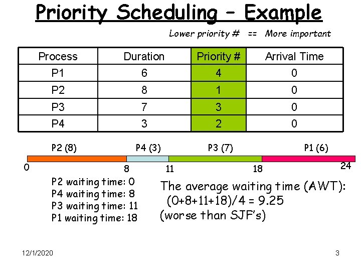
Priority Scheduling – Example Lower priority # == More important Process Duration Priority # Arrival Time P 1 6 4 0 P 2 8 1 0 P 3 7 3 0 P 4 3 2 0 P 2 (8) 0 P 4 (3) 8 P 2 waiting time: 0 P 4 waiting time: 8 P 3 waiting time: 11 P 1 waiting time: 18 12/1/2020 P 3 (7) 11 P 1 (6) 24 18 The average waiting time (AWT): (0+8+11+18)/4 = 9. 25 (worse than SJF’s) 3

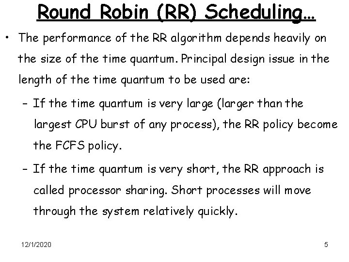
Round Robin (RR) Scheduling • RR is preemptive and designed especially for time sharing systems. • A clock interrupt is generated at periodic intervals called time quantum or time slice. • To implement RR scheduling, we keep the ready queue as a FIFO queue of processes. New processes are added to the tail of the ready queue. The CPU scheduler picks the first process, sets a timer to interrupt after 1 time quantum, and dispatches the process. • One of two things will then happen. The process may have a CPU burst of less than 1 time quantum. In this case, the process itself will release the CPU voluntarily. The scheduler will then proceed to the next process in the ready queue. Otherwise, if the CPU burst of the currently running process is greater than 1 time quantum; the timer will go off and will cause an interrupt to the operating system. A context switch will be executed, and the process will be put at the tail of the ready queue. The CPU scheduler will then select the next process from the ready queue. 12/1/2020 4

Round Robin (RR) Scheduling… • The performance of the RR algorithm depends heavily on the size of the time quantum. Principal design issue in the length of the time quantum to be used are: – If the time quantum is very large (larger than the largest CPU burst of any process), the RR policy become the FCFS policy. – If the time quantum is very short, the RR approach is called processor sharing. Short processes will move through the system relatively quickly. 12/1/2020 5

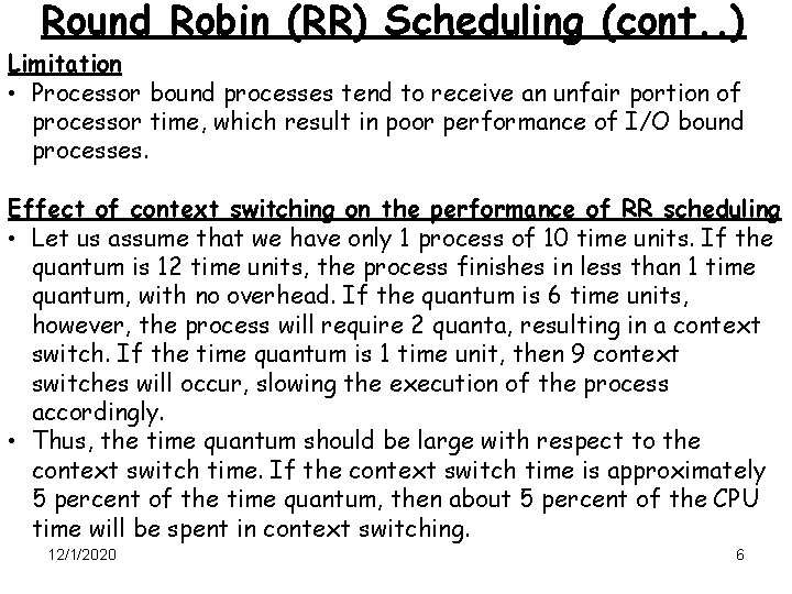
Round Robin (RR) Scheduling (cont. . ) Limitation • Processor bound processes tend to receive an unfair portion of processor time, which result in poor performance of I/O bound processes. Effect of context switching on the performance of RR scheduling • Let us assume that we have only 1 process of 10 time units. If the quantum is 12 time units, the process finishes in less than 1 time quantum, with no overhead. If the quantum is 6 time units, however, the process will require 2 quanta, resulting in a context switch. If the time quantum is 1 time unit, then 9 context switches will occur, slowing the execution of the process accordingly. • Thus, the time quantum should be large with respect to the context switch time. If the context switch time is approximately 5 percent of the time quantum, then about 5 percent of the CPU time will be spent in context switching. 12/1/2020 6

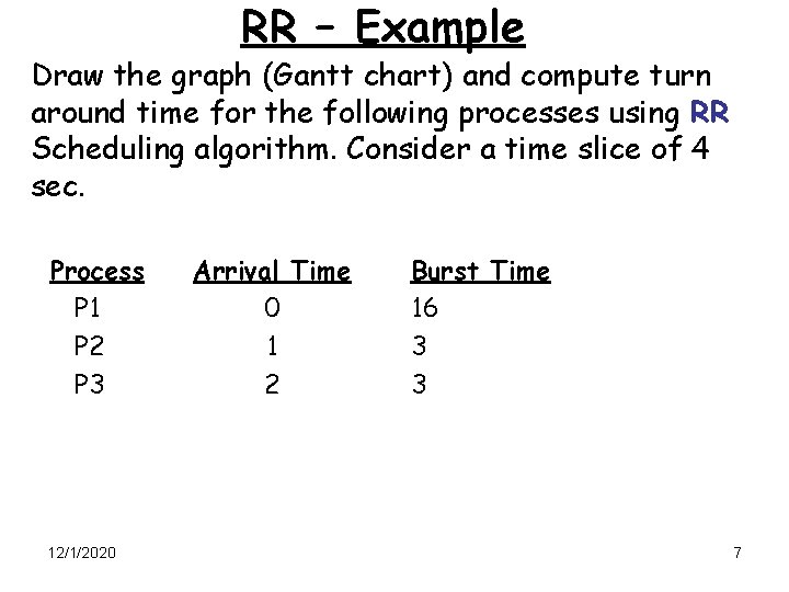
RR – Example Draw the graph (Gantt chart) and compute turn around time for the following processes using RR Scheduling algorithm. Consider a time slice of 4 sec. Process P 1 P 2 P 3 12/1/2020 Arrival Time 0 1 2 Burst Time 16 3 3 7

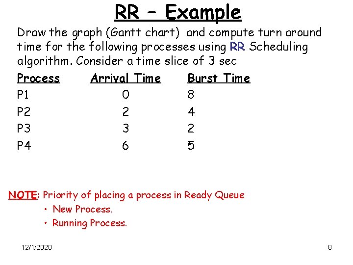
RR – Example Draw the graph (Gantt chart) and compute turn around time for the following processes using RR Scheduling algorithm. Consider a time slice of 3 sec Process Arrival Time Burst Time P 1 0 8 P 2 2 4 P 3 3 2 P 4 6 5 NOTE: Priority of placing a process in Ready Queue • New Process. • Running Process. 12/1/2020 8

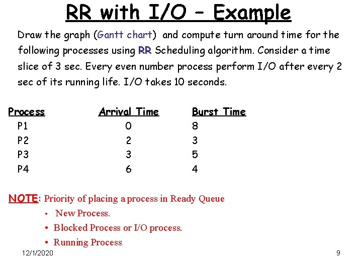
RR with I/O – Example Draw the graph (Gantt chart) and compute turn around time for the following processes using RR Scheduling algorithm. Consider a time slice of 3 sec. Every even number process perform I/O after every 2 sec of its running life. I/O takes 10 seconds. Process P 1 P 2 P 3 P 4 Arrival Time 0 2 3 6 Burst Time 8 3 5 4 NOTE: Priority of placing a process in Ready Queue • New Process. • Blocked Process or I/O process. • Running Process. 12/1/2020 9

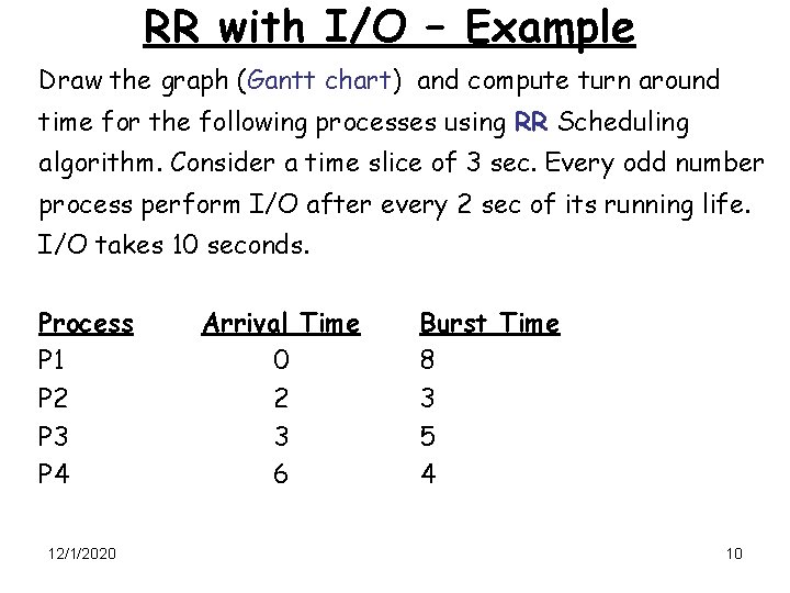
RR with I/O – Example Draw the graph (Gantt chart) and compute turn around time for the following processes using RR Scheduling algorithm. Consider a time slice of 3 sec. Every odd number process perform I/O after every 2 sec of its running life. I/O takes 10 seconds. Process P 1 P 2 P 3 P 4 12/1/2020 Arrival Time 0 2 3 6 Burst Time 8 3 5 4 10

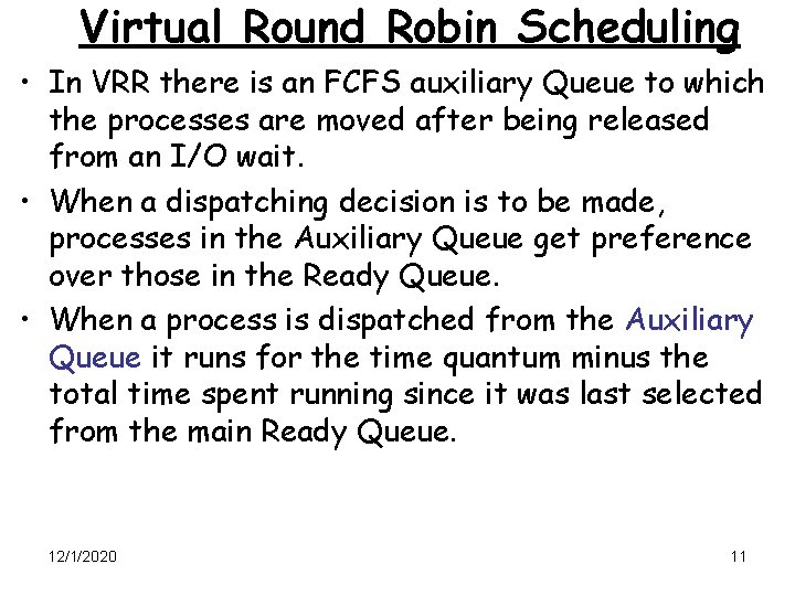
Virtual Round Robin Scheduling • In VRR there is an FCFS auxiliary Queue to which the processes are moved after being released from an I/O wait. • When a dispatching decision is to be made, processes in the Auxiliary Queue get preference over those in the Ready Queue. • When a process is dispatched from the Auxiliary Queue it runs for the time quantum minus the total time spent running since it was last selected from the main Ready Queue. 12/1/2020 11

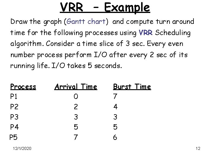
VRR – Example Draw the graph (Gantt chart) and compute turn around time for the following processes using VRR Scheduling algorithm. Consider a time slice of 3 sec. Every even number process perform I/O after every 2 sec of its running life. I/O takes 5 seconds. Process P 1 P 2 P 3 P 4 P 5 12/1/2020 Arrival Time 0 2 3 5 7 Burst Time 7 4 3 5 6 12

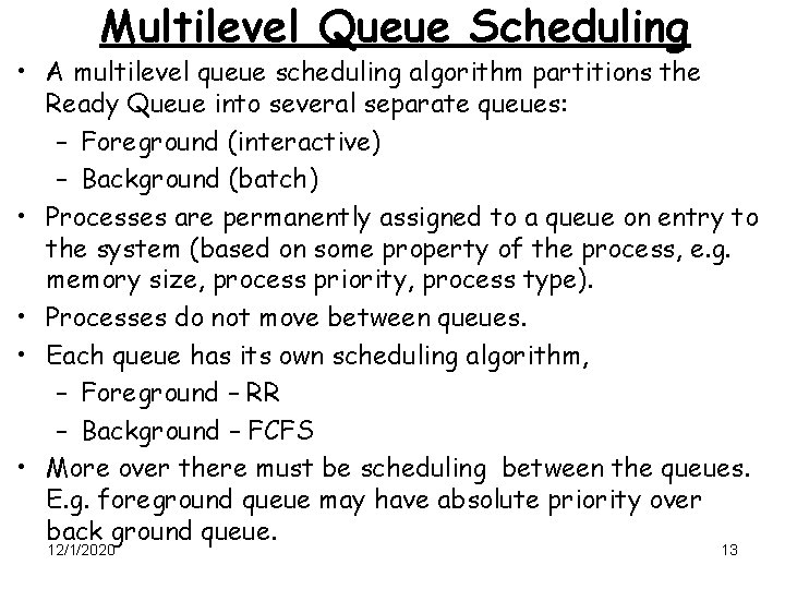
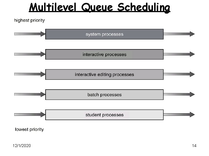
Multilevel Queue Scheduling • A multilevel queue scheduling algorithm partitions the Ready Queue into several separate queues: – Foreground (interactive) – Background (batch) • Processes are permanently assigned to a queue on entry to the system (based on some property of the process, e. g. memory size, process priority, process type). • Processes do not move between queues. • Each queue has its own scheduling algorithm, – Foreground – RR – Background – FCFS • More over there must be scheduling between the queues. E. g. foreground queue may have absolute priority over back ground queue. 12/1/2020 13

Multilevel Queue Scheduling 12/1/2020 14

MQ Scheduling – Example Draw the graph (Gantt chart) for the following processes using MQ Scheduling algorithm. If (CPU time < 4) then Q 1 (FCFS) else if (4 <= CPU time < 7) then Q 2 (FCFS) else Q 3 (FCFS) Process Arrival Time Burst Time P 1 0 8 P 2 2 2 P 3 3 4 P 4 5 6 P 5 7 9 P 6 9 3 P 7 10 5 12/1/2020 15

MQ Scheduling – Example Draw the graph (Gantt chart) for the following processes using MQ Scheduling algorithm. If (CPU time < 4) then Q 1 (FCFS) else if (4 <= CPU time < 7) then Q 2 (RR – 3 sec) else Q 3 (FCFS) Process P 1 P 2 P 3 P 4 P 5 P 6 P 7 12/1/2020 Arrival Time 0 2 3 5 7 9 10 Burst Time 8 2 4 6 9 3 5 16

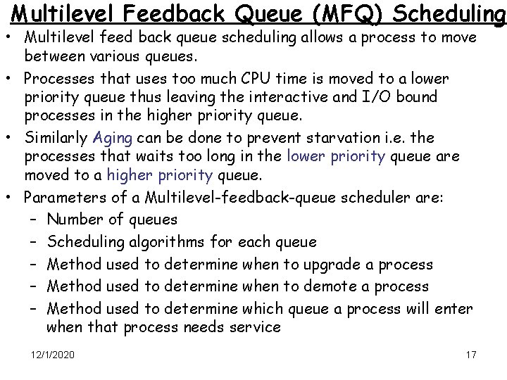
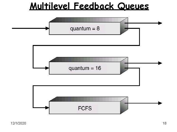
Multilevel Feedback Queue (MFQ) Scheduling • Multilevel feed back queue scheduling allows a process to move between various queues. • Processes that uses too much CPU time is moved to a lower priority queue thus leaving the interactive and I/O bound processes in the higher priority queue. • Similarly Aging can be done to prevent starvation i. e. the processes that waits too long in the lower priority queue are moved to a higher priority queue. • Parameters of a Multilevel-feedback-queue scheduler are: – Number of queues – Scheduling algorithms for each queue – Method used to determine when to upgrade a process – Method used to determine when to demote a process – Method used to determine which queue a process will enter when that process needs service 12/1/2020 17

Multilevel Feedback Queues 12/1/2020 18

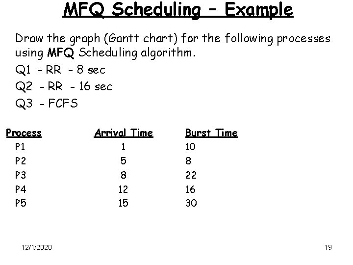
MFQ Scheduling – Example Draw the graph (Gantt chart) for the following processes using MFQ Scheduling algorithm. Q 1 - RR - 8 sec Q 2 - RR - 16 sec Q 3 - FCFS Process P 1 P 2 P 3 P 4 P 5 12/1/2020 Arrival Time 1 5 8 12 15 Burst Time 10 8 22 16 30 19

Evaluation of Scheduling Algorithms • Deterministic Modeling • Queuing Model • Simulation • Implementation 12/1/2020 20

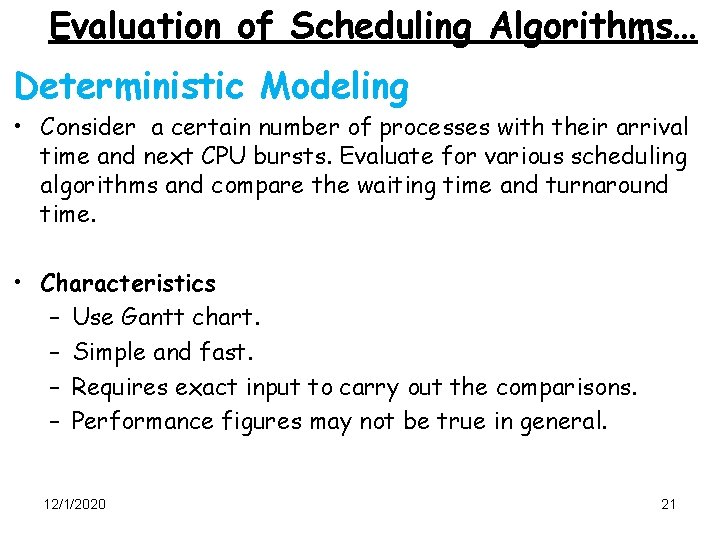
Evaluation of Scheduling Algorithms… Deterministic Modeling • Consider a certain number of processes with their arrival time and next CPU bursts. Evaluate for various scheduling algorithms and compare the waiting time and turnaround time. • Characteristics – Use Gantt chart. – Simple and fast. – Requires exact input to carry out the comparisons. – Performance figures may not be true in general. 12/1/2020 21

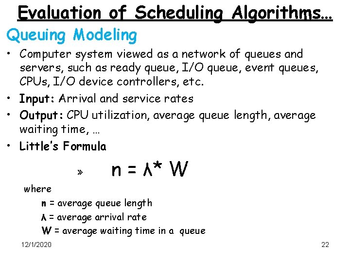
Evaluation of Scheduling Algorithms… Queuing Modeling • Computer system viewed as a network of queues and servers, such as ready queue, I/O queue, event queues, CPUs, I/O device controllers, etc. • Input: Arrival and service rates • Output: CPU utilization, average queue length, average waiting time, … • Little’s Formula » n = λ* W where n = average queue length λ = average arrival rate W = average waiting time in a queue 12/1/2020 22

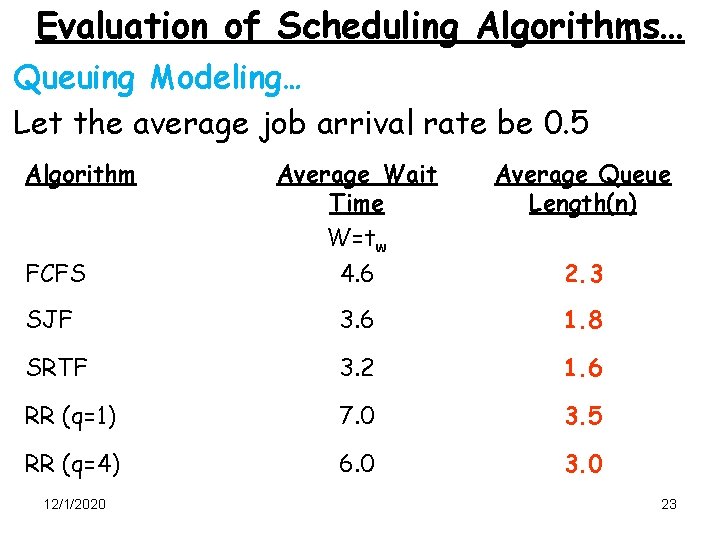
Evaluation of Scheduling Algorithms… Queuing Modeling… Let the average job arrival rate be 0. 5 Algorithm Average Queue Length(n) FCFS Average Wait Time W=tw 4. 6 SJF 3. 6 1. 8 SRTF 3. 2 1. 6 RR (q=1) 7. 0 3. 5 RR (q=4) 6. 0 3. 0 12/1/2020 2. 3 23

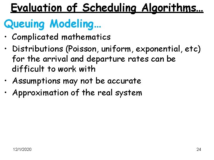
Evaluation of Scheduling Algorithms… Queuing Modeling… • Complicated mathematics • Distributions (Poisson, uniform, exponential, etc) for the arrival and departure rates can be difficult to work with • Assumptions may not be accurate • Approximation of the real system 12/1/2020 24

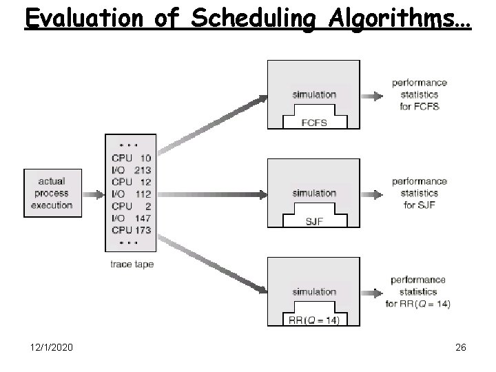
Evaluation of Scheduling Algorithms… Simulation § Programming model for the computer system § Workload random number generator, or by collecting data from the actual system. § Characteristics § Expensive: hours of programming and execution time § May be erroneous because of the assumptions about distributions § generated by assuming some distribution 12/1/2020 25

Evaluation of Scheduling Algorithms… Simulation 12/1/2020 26

Evaluation of Scheduling Algorithms… Implementation • If you have UNIX Kernel source code, use VMware change the code for scheduling, compile the Kernel again and test. • Characteristics – Most expensive – Good option due to Open Source kernels such as Linux 12/1/2020 27