Multilevel Models Multilevel modeling is a generalization of

Multilevel Models • Multilevel modeling is a generalization of regression methods. • Used for a variety of purposes, including prediction, data reduction, and causal inference. • From experiments and observational studies.

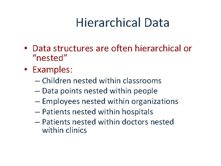
Hierarchical Data • Data structures are often hierarchical or “nested” • Examples: – Children nested within classrooms – Data points nested within people – Employees nested within organizations – Patients nested within hospitals – Patients nested within doctors nested within clinics Slide 2

Multilevel Models • Many names for similar models, analyses, and goals: • Multi-level model • Random effects model • Mixed model • Random coefficient model • Hierarchical model • Multilevel models are extensions of regression…

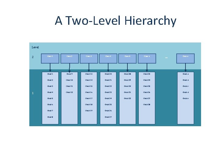
A Two-Level Hierarchy Level 2 1 Class 1 Class 2 Class 3 Class 4 Class 5 Class 6 Class n Child 1 Child 9 Child 13 Child 20 Child 28 Child 33 Child a Child 2 Child 10 Child 14 Child 21 Child 29 Child 34 Child b Child 3 Child 11 Child 15 Child 22 Child 30 Child 35 Child c Child 4 Child 12 Child 16 Child 23 Child 31 Child 36 Child d Child 32 Child 37 Child e . . . Child 5 Child 17 Child 24 Child 6 Child 18 Child 25 Child 7 Child 19 Child 26 Child 8 Child 27 Child 38

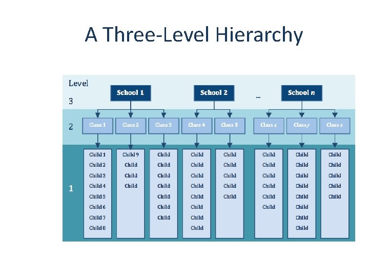
A Three-Level Hierarchy

Radon Example • I use an example from Gelman’s book: “Data Analysis Using Regression and Multilevel/Hierarchal Models” • Document the strengths and limitations of multilevel modeling.

Background • Effect of city-level policies on enforcing child support payments from unmarried fathers. • Treatment is at the group (city) level. • Outcome is measured on the individual family label.

Benefits of Multilevel Models • Homogeneity of regression slopes – Model the variability in regression slopes • Assumption of independence – You can model the relationships between cases – (Regression for repeated observations) • Missing data – MLMs can cope with missing data

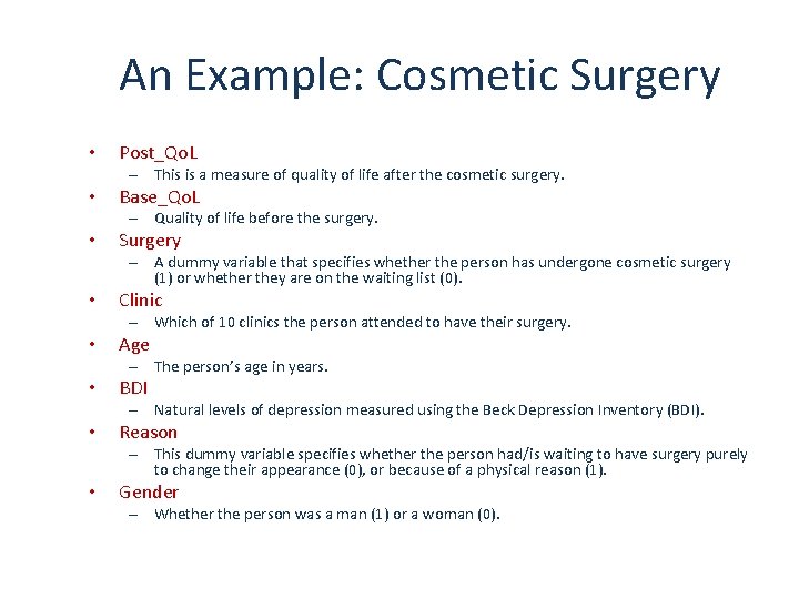
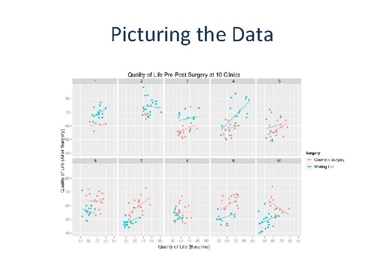
An Example: Cosmetic Surgery • Post_Qo. L – This is a measure of quality of life after the cosmetic surgery. • Base_Qo. L – Quality of life before the surgery. • Surgery – A dummy variable that specifies whether the person has undergone cosmetic surgery (1) or whether they are on the waiting list (0). • Clinic – Which of 10 clinics the person attended to have their surgery. • Age – The person’s age in years. • BDI – Natural levels of depression measured using the Beck Depression Inventory (BDI). • Reason – This dummy variable specifies whether the person had/is waiting to have surgery purely to change their appearance (0), or because of a physical reason (1). • Gender – Whether the person was a man (1) or a woman (0).

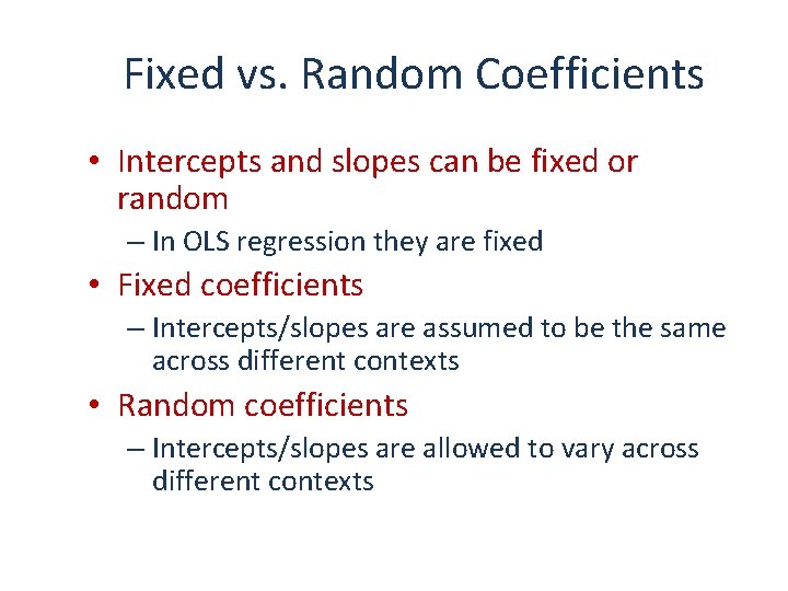
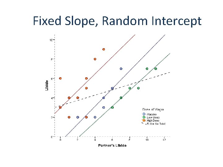
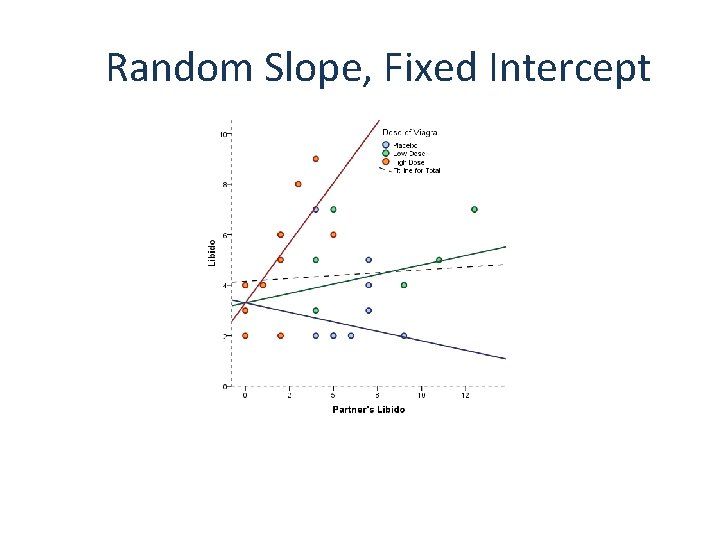
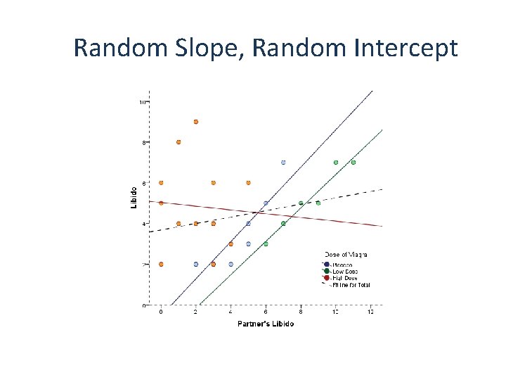
Fixed vs. Random Coefficients • Intercepts and slopes can be fixed or random – In OLS regression they are fixed • Fixed coefficients – Intercepts/slopes are assumed to be the same across different contexts • Random coefficients – Intercepts/slopes are allowed to vary across different contexts

Fixed Slope, Random Intercept

Random Slope, Fixed Intercept

Random Slope, Random Intercept

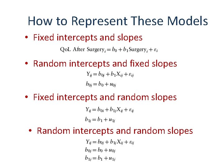
How to Represent These Models • Fixed intercepts and slopes • Random intercepts and fixed slopes • Fixed intercepts and random slopes • Random intercepts and random slopes

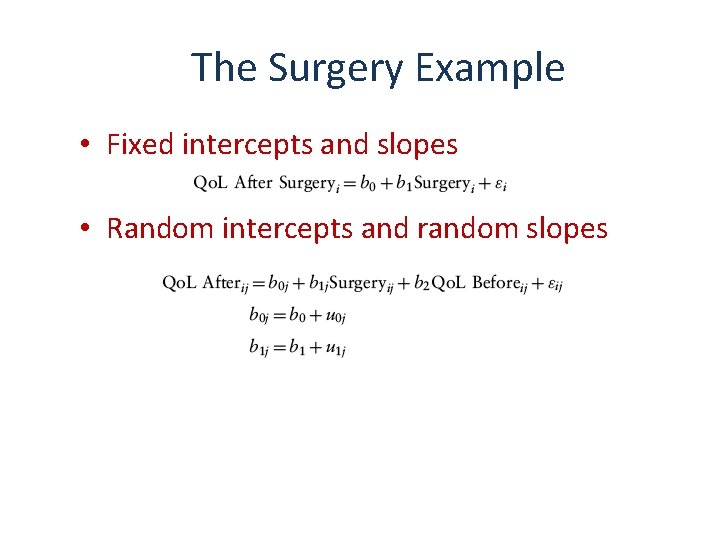
The Surgery Example • Fixed intercepts and slopes • Random intercepts and random slopes

Comparing Models • Models should be built up gradually – Start with fixed coefficients – Change one aspect of the model and compare to the previous with the change in the – 2 LL • Assessing fit – AIC – BIC

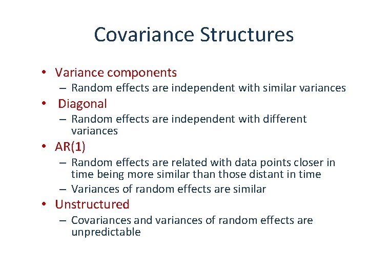
Covariance Structures • Variance components – Random effects are independent with similar variances • Diagonal – Random effects are independent with different variances • AR(1) – Random effects are related with data points closer in time being more similar than those distant in time – Variances of random effects are similar • Unstructured – Covariances and variances of random effects are unpredictable

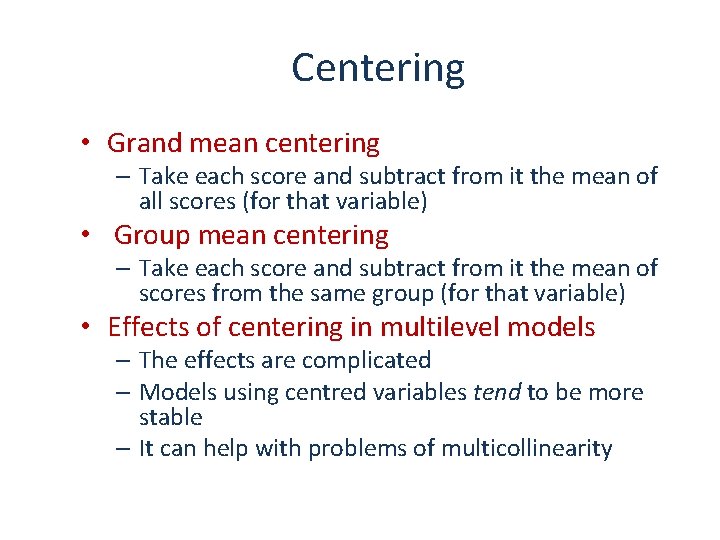
Centering • Grand mean centering – Take each score and subtract from it the mean of all scores (for that variable) • Group mean centering – Take each score and subtract from it the mean of scores from the same group (for that variable) • Effects of centering in multilevel models – The effects are complicated – Models using centred variables tend to be more stable – It can help with problems of multicollinearity

Picturing the Data

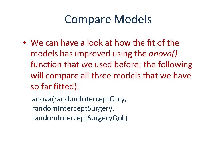
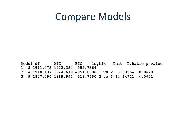
Compare Models • We can have a look at how the fit of the models has improved using the anova() function that we used before; the following will compare all three models that we have so far fitted): anova(random. Intercept. Only, random. Intercept. Surgery. Qo. L)

Compare Models

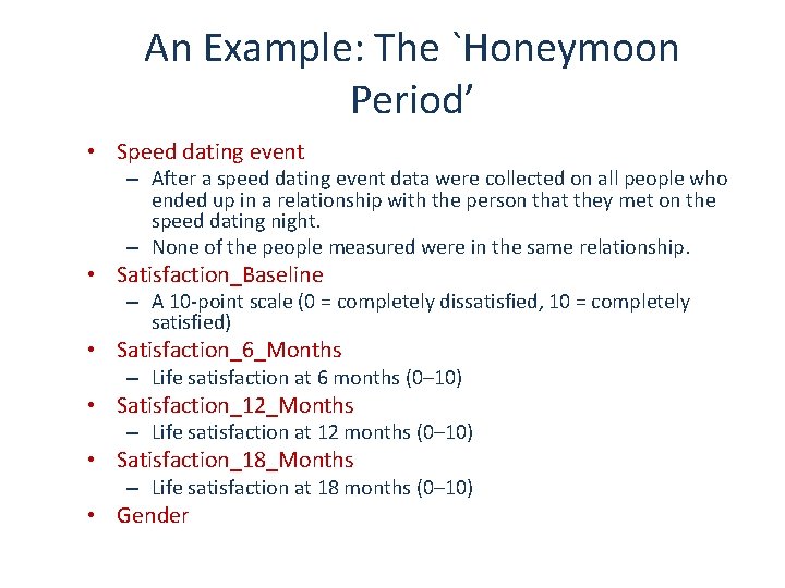
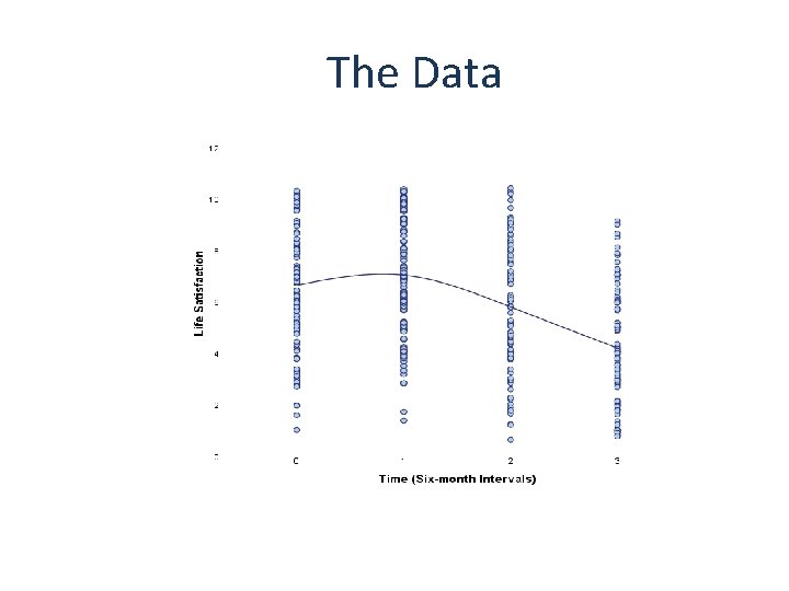
An Example: The `Honeymoon Period’ • Speed dating event – After a speed dating event data were collected on all people who ended up in a relationship with the person that they met on the speed dating night. – None of the people measured were in the same relationship. • Satisfaction_Baseline – A 10 -point scale (0 = completely dissatisfied, 10 = completely satisfied) • Satisfaction_6_Months – Life satisfaction at 6 months (0– 10) • Satisfaction_12_Months – Life satisfaction at 12 months (0– 10) • Satisfaction_18_Months – Life satisfaction at 18 months (0– 10) • Gender

The Data

Restructuring Data • Data entry for multilevel models … – Need the variable Time to be represented by a single column. We refer to this format as the ‘long’ format. As such we need to restructure the data. – But, in repeated measures designs we’re used to entering data so that instances of the outcome appear in different columns.

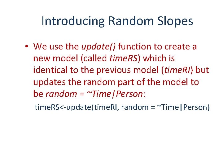
Introducing Random Slopes • We use the update() function to create a new model (called time. RS) which is identical to the previous model (time. RI) but updates the random part of the model to be random = ~Time|Person: time. RS<-update(time. RI, random = ~Time|Person)

To Sum Up … • Data can be hierarchical and this hierarchical structure can be important. – Most of the tests that you learn simply ignore the hierarchy. • Hierarchical models are just a fancy regression in which you can estimate the variability in the slopes and intercepts within entities. – Slopes and intercepts can be random variables (allowed to vary) rather than fixed (assumed to be equal in different situations). • Start with a model that ignores the hierarchy and then add in random intercepts and slopes to see if they improve the fit of the model. • Growth curves model trends in the data over time – These trends can also have variable intercepts and slopes. Slide 26