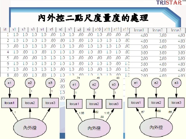
Best readings for SEM 2 Best readings for


Best readings for SEM 2

Best readings for SEM 3

Best readings for SEM 4


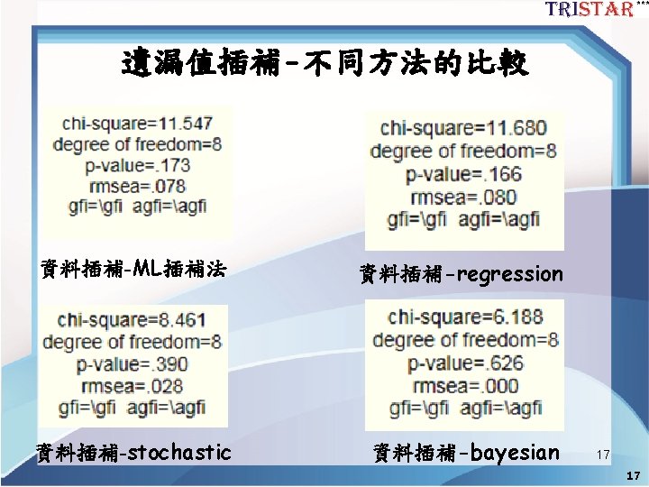
遺漏值插補-ML插補 • View Analysis Properties Estimate Mean and Intercept 打勾 分析 標準化輸出 13 13

遺漏值插補- Regression imputation • Analyze Data Imputation Regression imputation 14 14

遺漏值插補- Stochastic regression imputation • Analyze Data Imputation Stochastic regression imputation 15 15

遺漏值插補-Bayesian imputation • Analyze Data Imputation Bayesian imputation 16 16

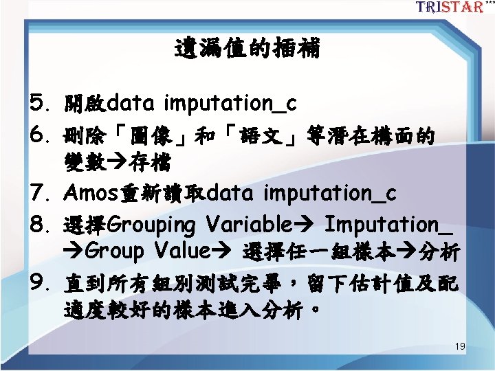
遺漏值的插補 1. View Interface Properties Estimate Means and Intercepts打勾 2. Analyze Data Imputation Bayesian imputation 3. 依右圖設定 4. 貝氏估計由綠色臉變成 黃色笑臉 表收斂完成 18

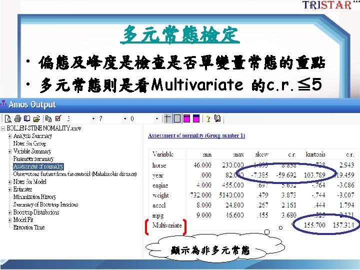
View Analysis Properties Output 22


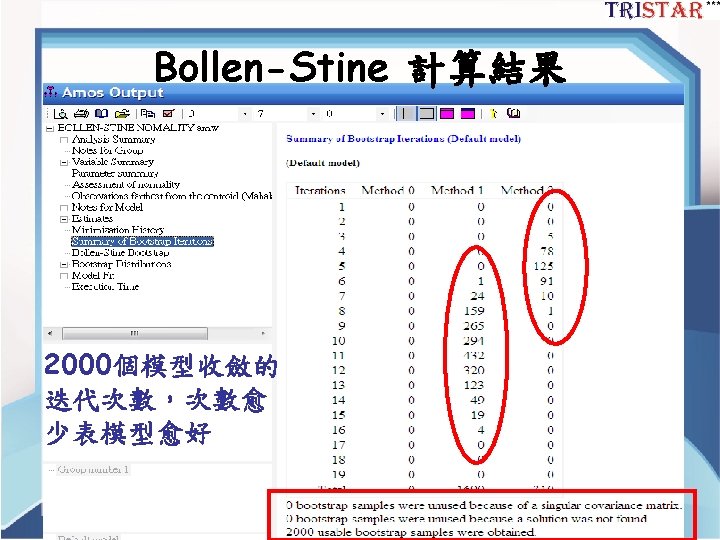
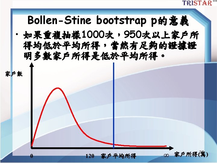
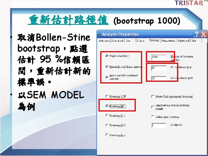
Bollen-Stine bootstrap • Bootstrap次數學者 建議 1000次~5000 次。 • Bollen-Stine建議採 2000次,一般不得 少於 1000次。 28
 • H 0: ML Χ 2 = Bollen-Stine")
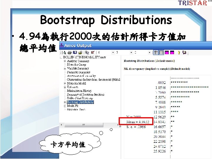
Bollen-Stine p-value correction (Byrne 2001, 284~285) • H 0: ML Χ 2 = Bollen-Stine Χ 2 估計的配適度一樣。 • P<0. 05表示ML與Bollen-Stine估計的Χ 2不同 • Bollen-Stine bootstrap p的意義為:下一個出 現較差模型的機率為(240+1)/2001= 0. 1204 30

SEM模型Bollen-Stine配適度修正 • Bollen-Stine bootstrap 2000次 32

33

Bollen-Stine p procedure correction 34


ML與Bootstrap估計值 • Bootstrap的表要在點選estimate下的選項後, 下面Bootstrap的結果才能點選 41

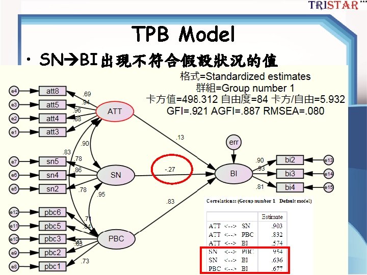
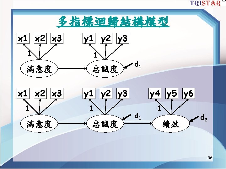
TPB結構模型 Figure 1. SEM結構模型 44

TPB的CFA Model 第一步:將模型重 新架構成一階CFA 完全有相關 Figure 2. TPB的CFA Model 45


如何解決模型中潛在變 項單一指標測量? O'Brien, Robert. 1994. "Identification of Simple Measurement Models with Multiple Latent Variables and Correlated Errors. " pp. 137 -170 in Peter Marsden (Ed. ) Sociological Methodology. Blackwell. 55

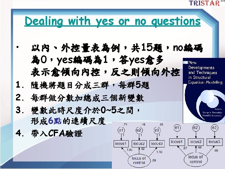
Two indicators rules 57
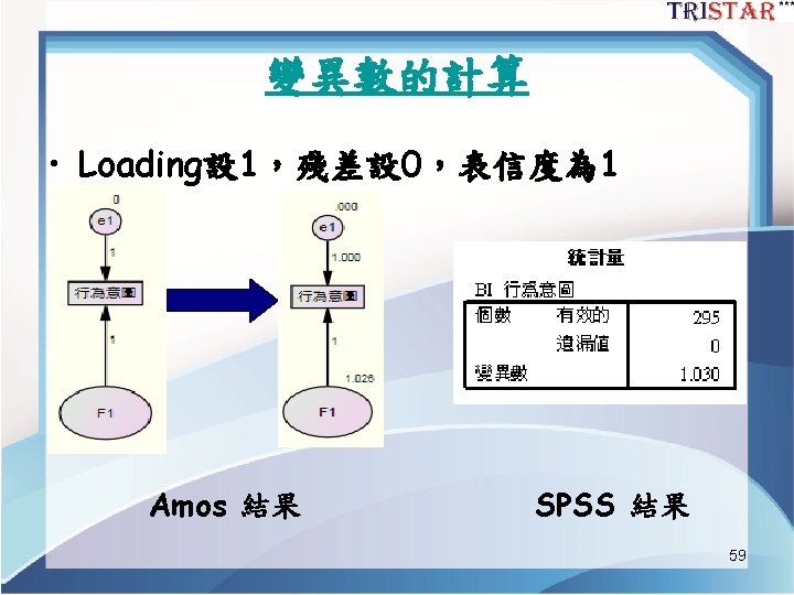
![潛在變數單一指標測量 1 F x 1 e • x=F+e Var(x)=Var(F)+Var(e) • 信度= Var(F)/Var(x) = [Var(x)-Var(e)]/Var(x)](http://slidetodoc.com/presentation_image_h/d188a2c3fe1254371076fe70cedbdef1/image-58.jpg "潛在變數單一指標測量 1 F x 1 e • x=F+e Var(x)=Var(F)+Var(e) • 信度= Var(F)/Var(x) = [Var(x)-Var(e)]/Var(x)")
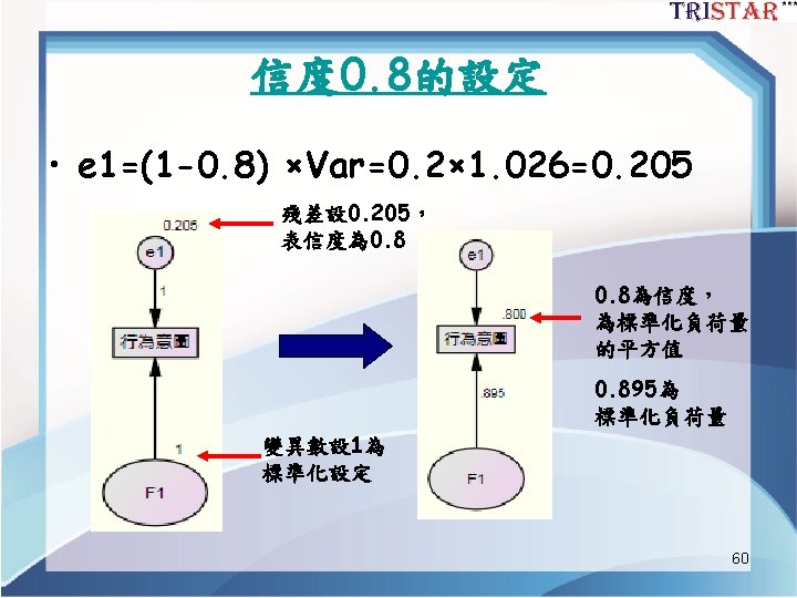
潛在變數單一指標測量 1 F x 1 e • x=F+e Var(x)=Var(F)+Var(e) • 信度= Var(F)/Var(x) = [Var(x)-Var(e)]/Var(x) =1 - Var(e)/Var(x) • Var(e)=(1 -信度) × Var(x) 58

Item parceling 61


SEM TAM Parceling TAM 63
α Var(x)(1 -α) ATT 0. 75")
因素負荷量與測量誤差 Variable α λ= Error= 1 -α Variance √Var(x)α Var(x)(1 -α) ATT 0. 75 0. 25 1. 004 0. 868 0. 251 EOU 0. 784 0. 216 0. 715 0. 749 0. 154 UF 0. 758 0. 242 0. 833 0. 795 0. 202 BI 0. 888 0. 112 1. 030 0. 956 0. 115 64

SEM TAM Parceling TAM 65


polychoric 或 polyserial matrics • 利用lisrel的prelis語法轉出適當的矩陣 68

SEM相關矩陣的應用 1. Both vars interval: Pearson r 2. Both vars dichotomous: Tetrachoric correlation 3. Both vars ordinal: Polychoric correlation 4. One var interval, the other a force dichotomy: Biserial correlation 69

SEM相關矩陣的應用 5. One var interval, the other ordinal: Polyserial correlation 6. One var interval, the other a true dichotomy: point-biserial 7. Both true ordinal: Spearman rank correlation or Kendall’s tau 8. Both true nominal: phi or contingency coefficient 9. One true ordinal, one true nominal: gamma 70

SEM相關矩陣 interval ordinal interval Pearson r ordinal Polychoric polyserial Spearman or Kendall nominal Biserial Polybiserial gamma nominal Tetrachoric Phi or contigency 71


73

74

的介紹及重要性 Power & sample sizes decision Satorra & Sarris (1985) Mac.")
結構方程模型的檢定力計算及 樣本數決定 檢定力 (power)的介紹及重要性 Power & sample sizes decision Satorra & Sarris (1985) Mac. Callum, Browne & Sugawara (1996) 78
 Type I error A false alarm Type II")
型I與型II錯誤 (Type I and II error) Type I error A false alarm Type II error A missed detection 無中生有 失之交臂 80

Effect size vs. power • Effect size愈大,power愈大 81


 Ha: εa= 0. 08 •")
檢定力的假設 • H 0: ε≦ 0. 05 (close fit) Ha: εa= 0. 08 • H 0: ε≧ 0. 05 (not-close fit) Ha: εa= 0. 01 88

R語言執行SEM 檢定統計力 #Power analysis for SEM alpha <- 0. 05 #alpha level d <- 200 #degrees of freedom n <- 250 #sample size rmsea 0 <- 0. 05 #null hypothesized RMSEA rmseaa <- 0. 08 #alternative hypothesized RMSEA #Code below this point need not be changed by user ncp 0 <- (n-1)*d*rmsea 0^2 ncpa <- (n-1)*d*rmseaa^2 #Compute power if(rmsea 0<rmseaa) { cval <qchisq(alpha, d, ncp=ncp 0, lower. tail=F) pow <pchisq(cval, d, ncp=ncpa, lower. t ail=F) } if(rmsea 0>rmseaa) { cval <- qchisq(1 alpha, d, ncp=ncp 0, lower. tail=F) pow <- 1 pchisq(cval, d, ncp=ncpa, lower. t ail=F) } print(pow) 89

R語言計算SEM 樣本數 #Computation of minimum sample size for test of fit rmsea 0 <- 0. 05 #null hypothesized RMSEA rmseaa <- 0. 01 #alternative hypothesized RMSEA d <- 200 #degrees of freedom alpha <- 0. 05 #alpha level desired <- 0. 8 #desired power #Code below need not be changed by user #initialize values pow <- 0. 0 n <- 0 #begin loop for finding initial level of n while (pow<desired) { n <- n+100 ncp 0 <- (n-1)*d*rmsea 0^2 ncpa <- (n-1)*d*rmseaa^2 #compute power if(rmsea 0<rmseaa) { cval <qchisq(alpha, d, ncp=ncp 0, lower. tail =F) pow <pchisq(cval, d, ncp=ncpa, lower. tail= F) } else { cval <- qchisq(1 alpha, d, ncp=ncp 0, lower. tail=F) pow <- 1 pchisq(cval, d, ncp=ncpa, lower. tail= F) }} 90

R語言計算SEM 樣本數 } #begin loop for interval halving else { foo <- -1 cval <- qchisq(1 newn <- n alpha, d, ncp=ncp 0, lower. tail=F) interval <- 200 pow <- 1 powdiff <- pow - desired pchisq(cval, d, ncp=ncpa, lower. tail=F while (powdiff>. 001) { ) interval <- interval*. 5 } newn <- newn + foo*interval*. 5 powdiff <- abs(pow-desired) ncp 0 <- (newn-1)*d*rmsea 0^2 if (pow<desired) { ncpa <- (newn-1)*d*rmseaa^2 foo <- 1 #compute power } if(rmsea 0<rmseaa) { if (pow>desired) { cval <foo <- -1 qchisq(alpha, d, ncp=ncp 0, lower. ta }} il=F) minn <- newn pow <pchisq(cval, d, ncp=ncpa, lower. print(minn) tail=F) 91


Jackson and Gillaspy, 2009 109

110
- Slides: 110