Markets and Algorithmic Game Theory the PrimalDual Paradigm

Markets and Algorithmic Game Theory the Primal-Dual Paradigm and Internet Computing Vijay V. Vazirani

Markets

Stock Markets

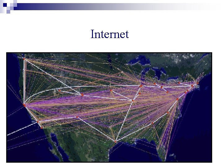
Internet

n Revolution in definition of markets

n Revolution in definition of markets n New markets defined by ¨ Google ¨ Amazon ¨ Yahoo! ¨ Ebay

n Revolution in definition of markets n Massive computational power available for running these markets in a centralized or distributed manner

n Revolution in definition of markets n Massive computational power available for running these markets in a centralized or distributed manner n Important to find good models and algorithms for these markets

Theory of Algorithms n Powerful tools and techniques developed over last 4 decades.

Theory of Algorithms n Powerful tools and techniques developed over last 4 decades. n Recent study of markets has contributed handsomely to this theory as well!

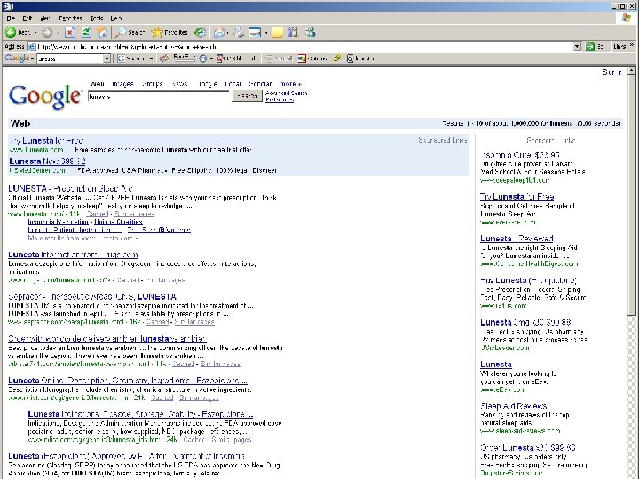
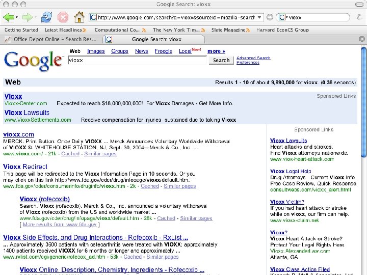
Ad. Words Market n Created by search engine companies ¨ Google ¨ Yahoo! ¨ MSN n Multi-billion dollar market – and still growing! n Totally revolutionized advertising, especially by small companies.

Historically, the study of markets n has been of central importance, especially in the West

Historically, the study of markets n has been of central importance, especially in the West General Equilibrium Theory Occupied center stage in Mathematical Economics for over a century

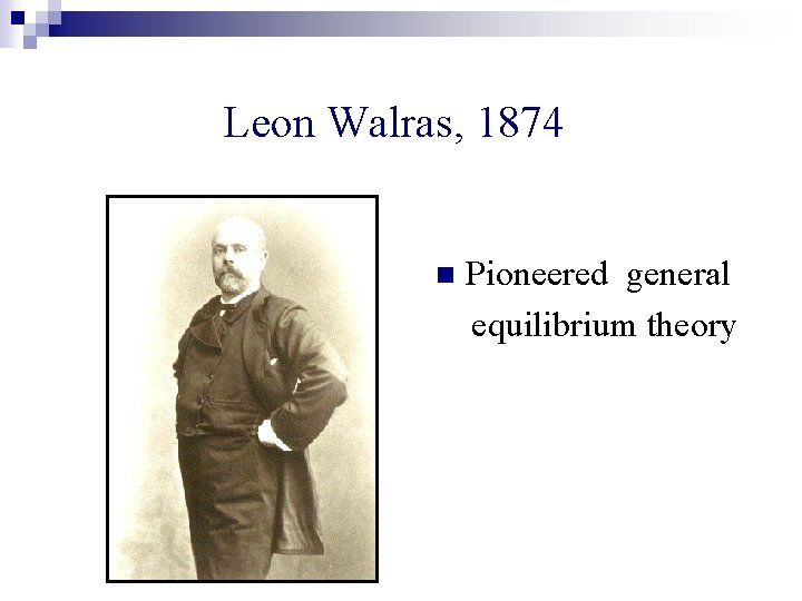
Leon Walras, 1874 n Pioneered general equilibrium theory

Arrow-Debreu Theorem, 1954 n Celebrated theorem in Mathematical Economics n Established existence of market equilibrium under very general conditions using a deep theorem from topology - Kakutani fixed point theorem.

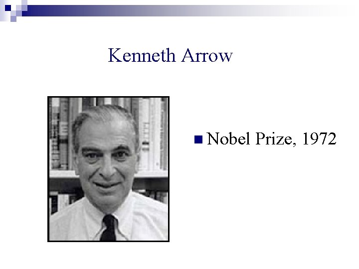
Kenneth Arrow n Nobel Prize, 1972

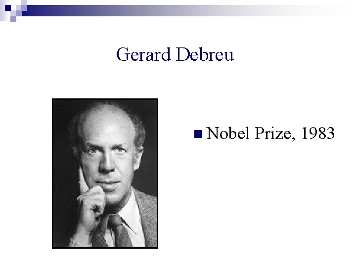
Gerard Debreu n Nobel Prize, 1983

General Equilibrium Theory n Also gave us some algorithmic results ¨ Convex programs, whose optimal solutions capture equilibrium allocations, e. g. , Eisenberg & Gale, 1959 Nenakov & Primak, 1983 ¨ Cottle and Eaves, 1960’s: Linear complimentarity ¨ Scarf, 1973: Algorithms for approximately computing fixed points

General Equilibrium Theory An almost entirely non-algorithmic theory!

What is needed today? n An inherently algorithmic theory of market equilibrium n New models that capture new markets and are easier to use than traditional models

n Beginnings of such a theory, within Algorithmic Game Theory n Started with combinatorial algorithms for traditional market models n New market models emerging

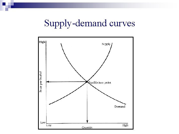
A central tenet n Prices are such that demand equals supply, i. e. , equilibrium prices.

A central tenet n Prices are such that demand equals supply, i. e. , equilibrium prices. n Easy if only one good

Supply-demand curves

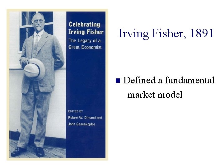
Irving Fisher, 1891 n Defined a fundamental market model

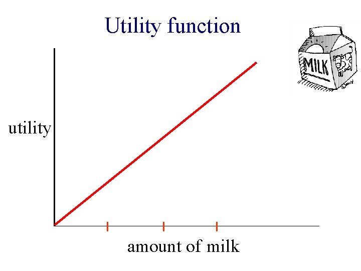
Utility function utility amount of milk

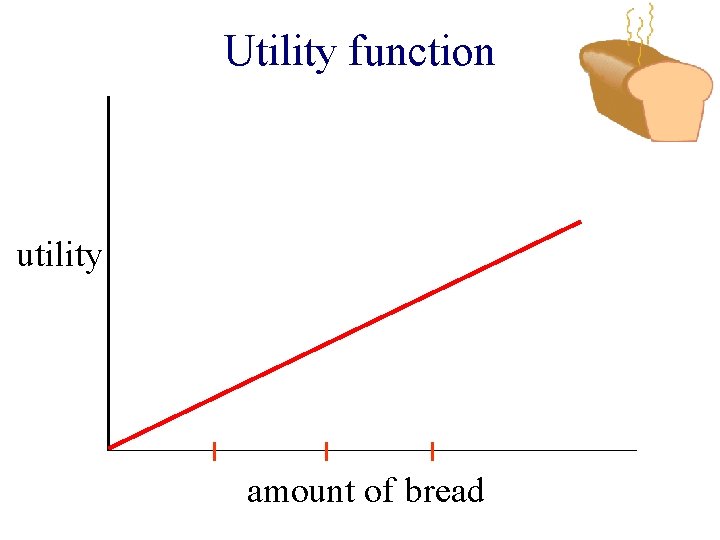
Utility function utility amount of bread

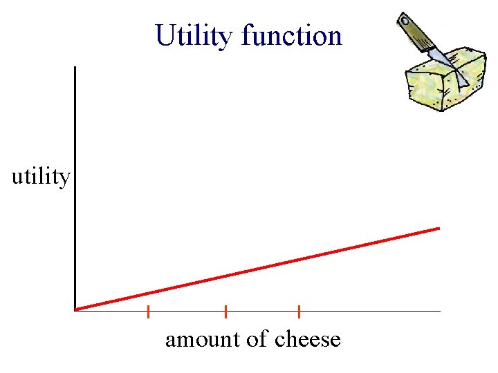
Utility function utility amount of cheese

Total utility of a bundle of goods = Sum of utilities of individual goods

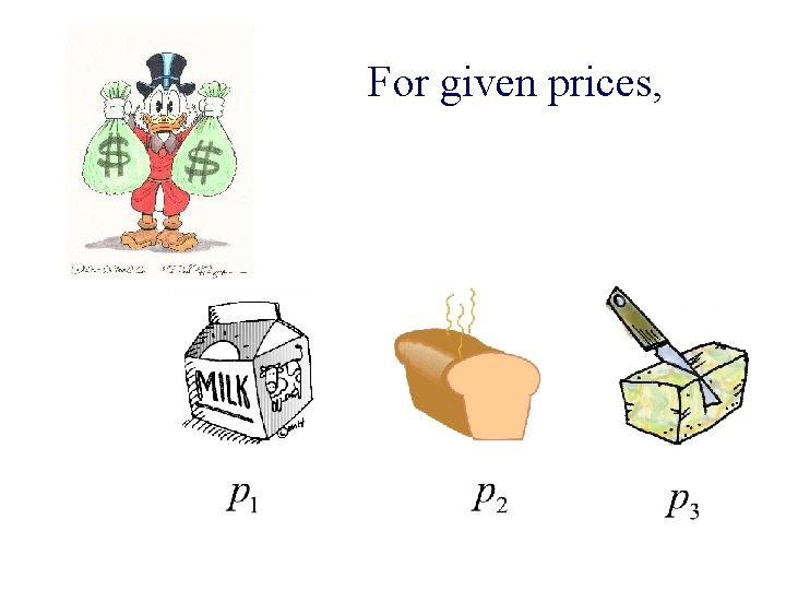
For given prices,

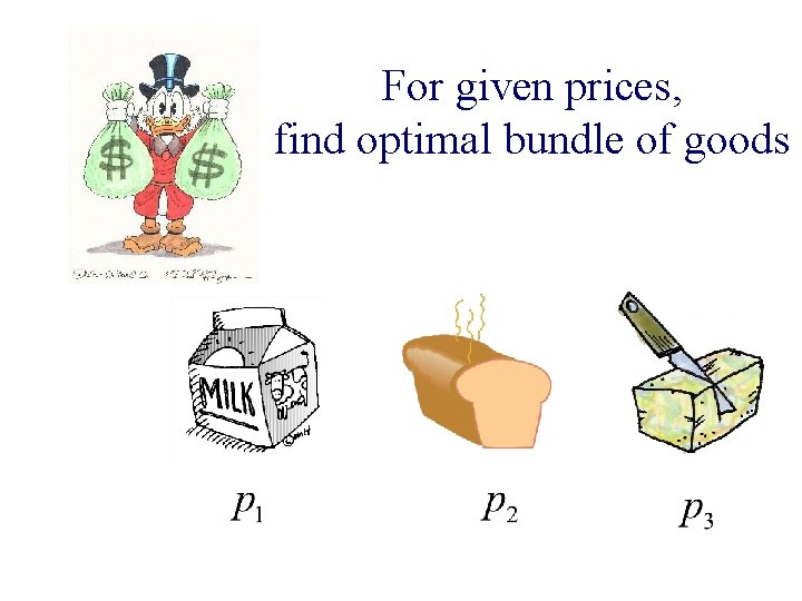
For given prices, find optimal bundle of goods

Fisher market n Several goods, fixed amount of each good n Several buyers, with individual money and utilities n Find equilibrium prices of goods, i. e. , prices s. t. , ¨ Each buyer gets an optimal bundle ¨ No deficiency or surplus of any good

Combinatorial Algorithm for Linear Case of Fisher’s Model n Devanur, Papadimitriou, Saberi & V. , 2002 Using the primal-dual schema

Primal-Dual Schema n Highly successful algorithm design technique from exact and approximation algorithms

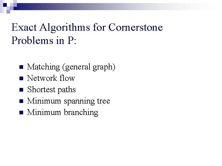
Exact Algorithms for Cornerstone Problems in P: n n n Matching (general graph) Network flow Shortest paths Minimum spanning tree Minimum branching

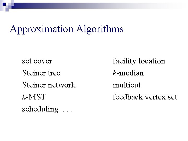
Approximation Algorithms set cover Steiner tree Steiner network k-MST scheduling. . . facility location k-median multicut feedback vertex set

n No LP’s known for capturing equilibrium allocations for Fisher’s model

n No LP’s known for capturing equilibrium allocations for Fisher’s model n Eisenberg-Gale convex program, 1959

n No LP’s known for capturing equilibrium allocations for Fisher’s model n Eisenberg-Gale convex program, 1959 n DPSV: Extended primal-dual schema to solving a nonlinear convex program

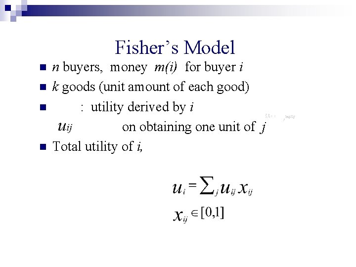
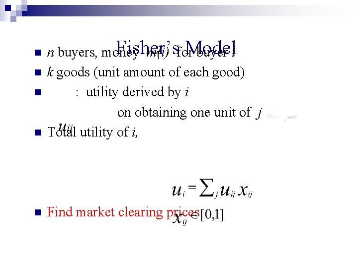
Fisher’s Model n n n buyers, money m(i) for buyer i k goods (unit amount of each good) : utility derived by i on obtaining one unit of j Total utility of i,

n Fisher’s Model n buyers, money m(i) for buyer i k goods (unit amount of each good) : utility derived by i on obtaining one unit of j Total utility of i, n Find market clearing prices n n n

An easier question n Given prices p, are they equilibrium prices? n If so, find equilibrium allocations.

An easier question n Given prices p, are they equilibrium prices? n If so, find equilibrium allocations. n Equilibrium prices are unique!

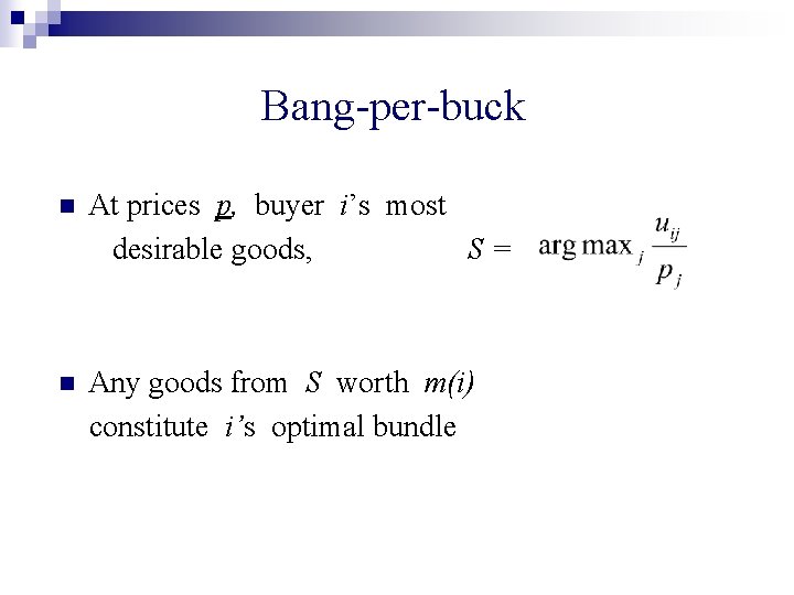
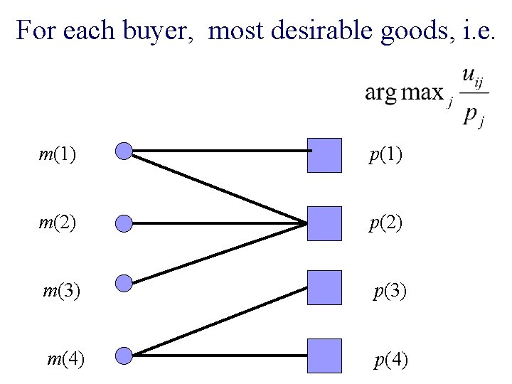
Bang-per-buck n At prices p, buyer i’s most desirable goods, S= n Any goods from S worth m(i) constitute i’s optimal bundle

For each buyer, most desirable goods, i. e. m(1) p(1) m(2) p(2) m(3) p(3) m(4) p(4)

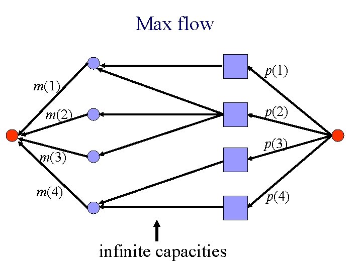
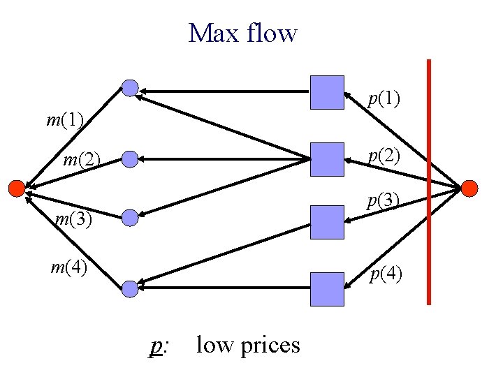
Max flow p(1) m(1) p(2) m(2) p(3) m(4) p(4) infinite capacities

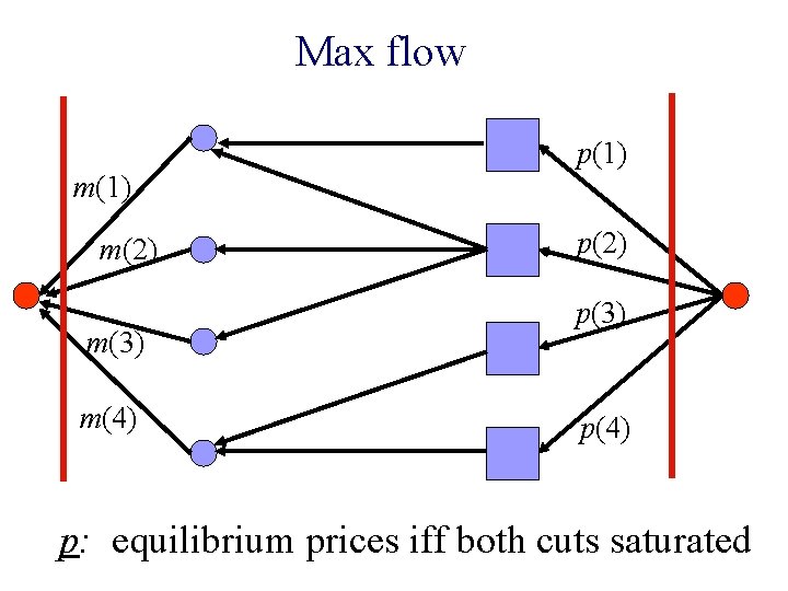
Max flow m(1) m(2) m(3) m(4) p(1) p(2) p(3) p(4) p: equilibrium prices iff both cuts saturated

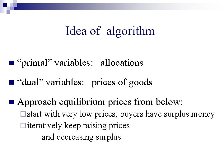
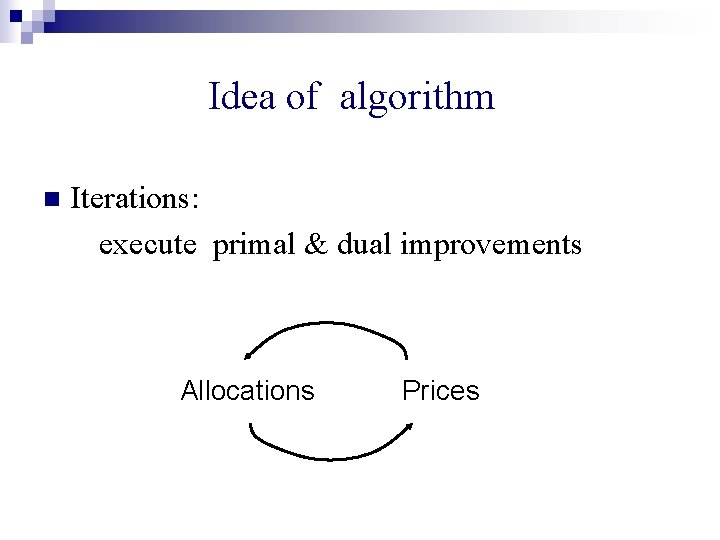
Idea of algorithm n “primal” variables: allocations n “dual” variables: prices of goods n Approach equilibrium prices from below: ¨ start with very low prices; buyers have surplus money ¨ iteratively keep raising prices and decreasing surplus

Idea of algorithm n Iterations: execute primal & dual improvements Allocations Prices

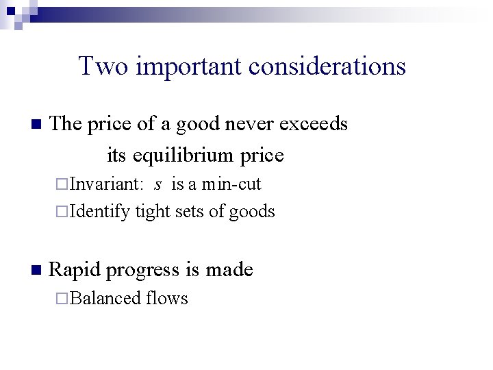
Two important considerations n The price of a good never exceeds its equilibrium price ¨ Invariant: s is a min-cut

Max flow p(1) m(1) p(2) m(2) p(3) m(4) p: low prices

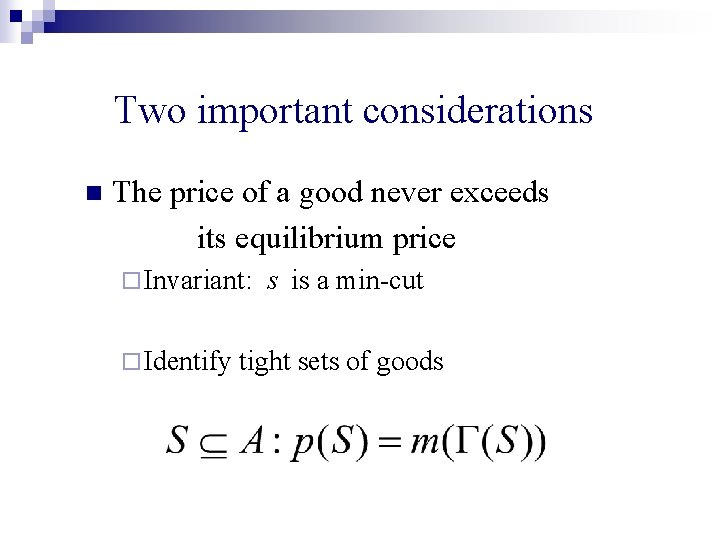
Two important considerations n The price of a good never exceeds its equilibrium price ¨ Invariant: ¨ Identify s is a min-cut tight sets of goods

Two important considerations n The price of a good never exceeds its equilibrium price ¨ Invariant: s is a min-cut ¨ Identify tight sets of goods n Rapid progress is made ¨ Balanced flows

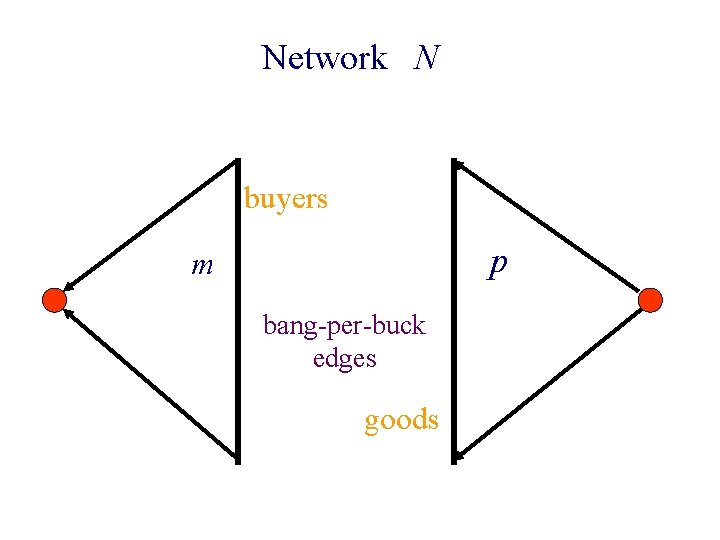
Network N buyers p m bang-per-buck edges goods

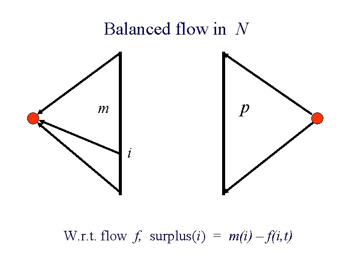
Balanced flow in N p m i W. r. t. flow f, surplus(i) = m(i) – f(i, t)

Balanced flow n surplus vector: vector of surpluses w. r. t. f.

Balanced flow n surplus vector: vector of surpluses w. r. t. f. n A flow that minimizes l 2 norm of surplus vector.

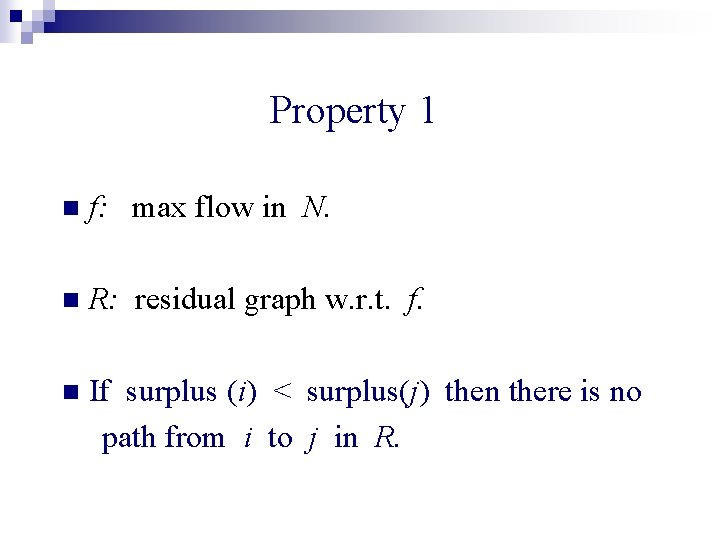
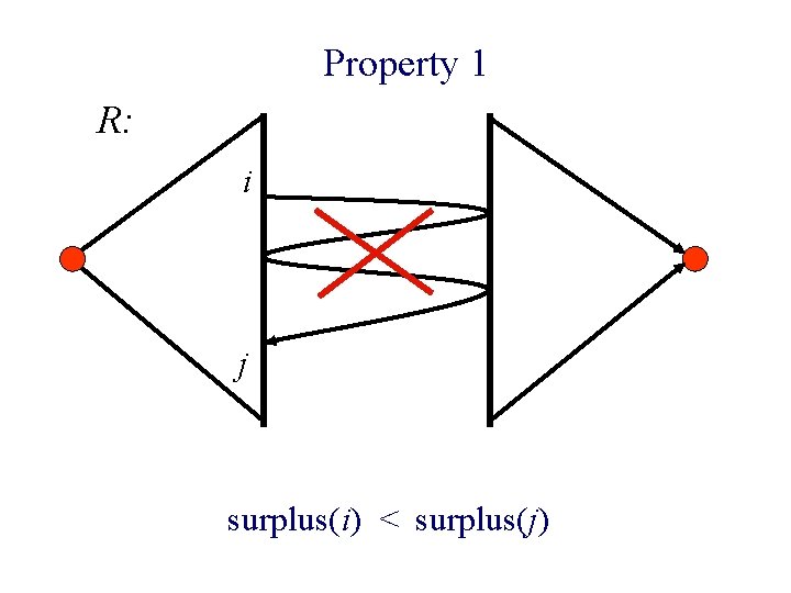
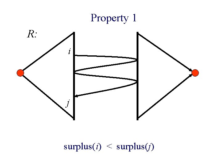
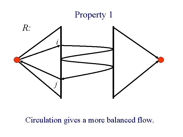
Property 1 n f: max flow in N. n R: residual graph w. r. t. f. n If surplus (i) < surplus(j) then there is no path from i to j in R.

Property 1 R: i j surplus(i) < surplus(j)

Property 1 R: i j surplus(i) < surplus(j)

Property 1 R: i j Circulation gives a more balanced flow.

Property 1 n Theorem: A max-flow is balanced iff it satisfies Property 1.

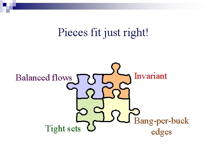
Pieces fit just right! Balanced flows Tight sets Invariant Bang-per-buck edges

How primal-dual schema is adapted to nonlinear setting

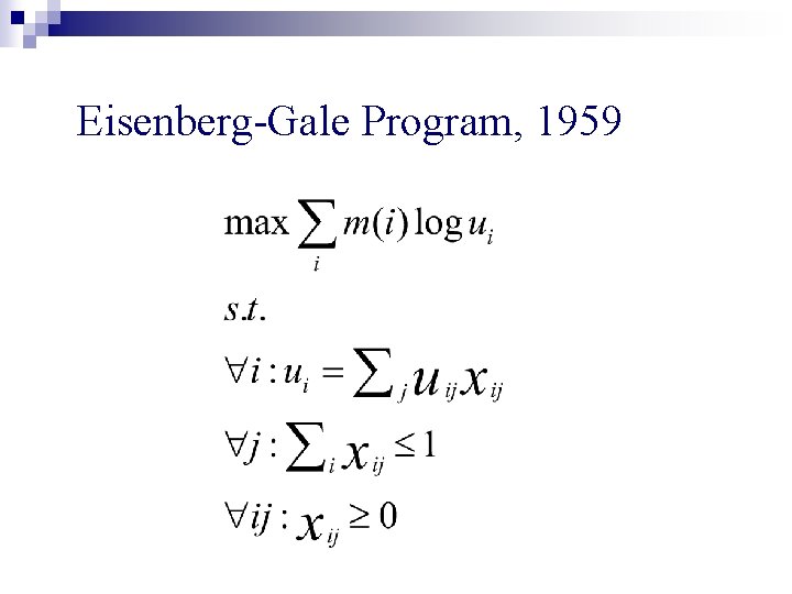
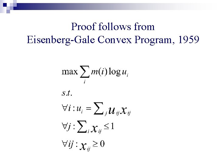
A convex program n whose optimal solution is equilibrium allocations.

A convex program n whose optimal solution is equilibrium allocations. n Constraints: packing constraints on the xij’s

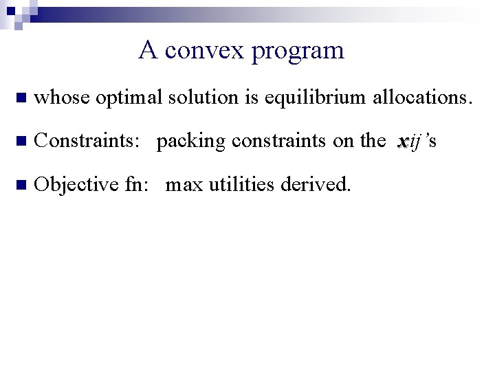
A convex program n whose optimal solution is equilibrium allocations. n Constraints: packing constraints on the xij’s n Objective fn: max utilities derived.

A convex program n whose optimal solution is equilibrium allocations. n Constraints: packing constraints on the xij’s n Objective fn: max utilities derived. Must satisfy ¨ If utilities of a buyer are scaled by a constant, optimal allocations remain unchanged ¨ If money of buyer b is split among two new buyers, whose utility fns same as b, then union of optimal allocations to new buyers = optimal allocation for b

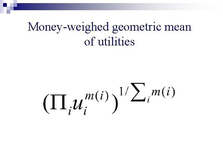
Money-weighed geometric mean of utilities

Eisenberg-Gale Program, 1959

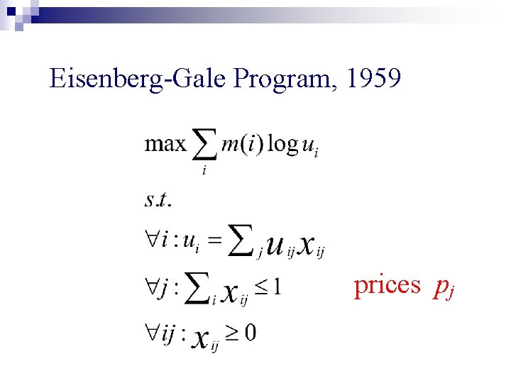
Eisenberg-Gale Program, 1959 prices pj

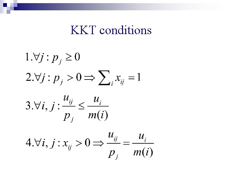
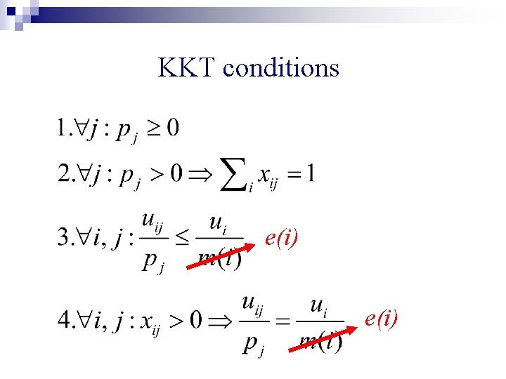
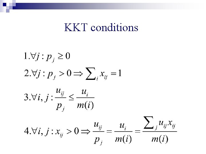
KKT conditions

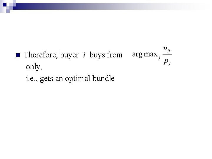
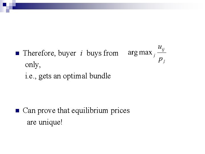
n Therefore, buyer i buys from only, i. e. , gets an optimal bundle

n Therefore, buyer i buys from only, i. e. , gets an optimal bundle n Can prove that equilibrium prices are unique!

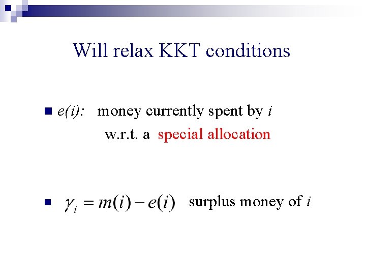
Will relax KKT conditions n n e(i): money currently spent by i w. r. t. a special allocation surplus money of i

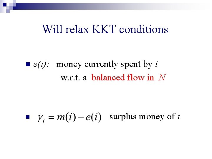
Will relax KKT conditions n n e(i): money currently spent by i w. r. t. a balanced flow in N surplus money of i

KKT conditions e(i)

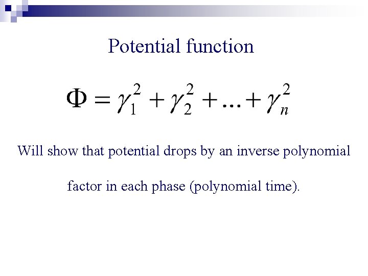
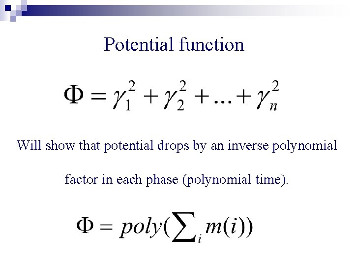
Potential function Will show that potential drops by an inverse polynomial factor in each phase (polynomial time).

Potential function Will show that potential drops by an inverse polynomial factor in each phase (polynomial time).

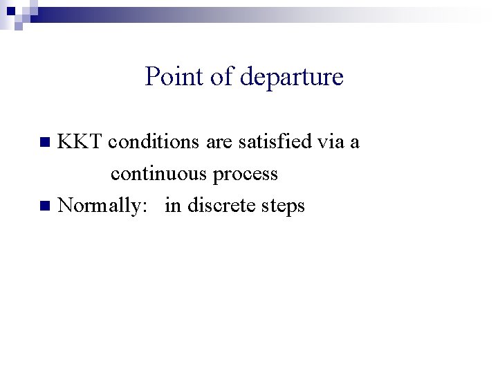
Point of departure KKT conditions are satisfied via a continuous process n Normally: in discrete steps n

Point of departure KKT conditions are satisfied via a continuous process n Normally: in discrete steps n n Open question: strongly polynomial algorithm?

Another point of departure n Complementary slackness conditions: involve primal or dual variables, not both. n KKT conditions: involve primal and dual variables simultaneously.

KKT conditions

KKT conditions

Primal-dual algorithms so far n Raise dual variables greedily. (Lot of effort spent on designing more sophisticated dual processes. )

Primal-dual algorithms so far n Raise dual variables greedily. (Lot of effort spent on designing more sophisticated dual processes. ) ¨ Only exception: Edmonds, 1965: algorithm for weight matching.

Primal-dual algorithms so far n Raise dual variables greedily. (Lot of effort spent on designing more sophisticated dual processes. ) ¨ Only n exception: Edmonds, 1965: algorithm for weight matching. Otherwise primal objects go tight and loose. Difficult to account for these reversals in the running time.

Our algorithm n Dual variables (prices) are raised greedily n Yet, primal objects go tight and loose ¨ Because of enhanced KKT conditions

Deficiencies of linear utility functions n Typically, a buyer spends all her money on a single good n Do not model the fact that buyers get satiated with goods

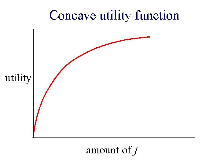
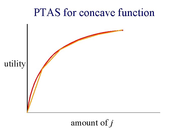
Concave utility function utility amount of j

Concave utility functions n Do not satisfy weak gross substitutability

Concave utility functions n Do not satisfy weak gross substitutability ¨ w. g. s. = Raising the price of one good cannot lead to a decrease in demand of another good.

Concave utility functions n Do not satisfy weak gross substitutability ¨ w. g. s. n = Raising the price of one good cannot lead to a decrease in demand of another good. Open problem: find polynomial time algorithm!

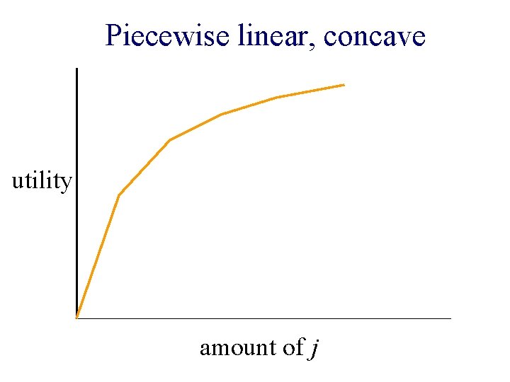
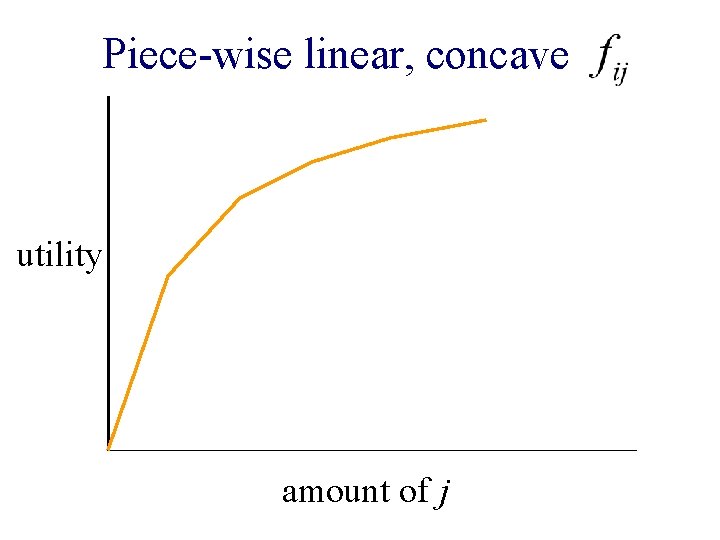
Piecewise linear, concave utility amount of j

PTAS for concave function utility amount of j

Piecewise linear concave utility n Does not satisfy weak gross substitutability

Piecewise linear, concave utility amount of j

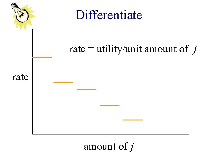
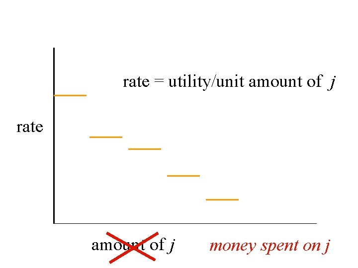
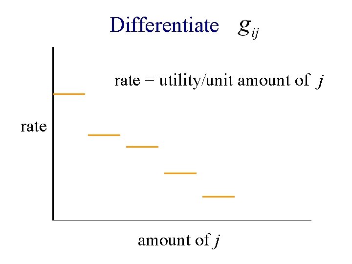
Differentiate rate = utility/unit amount of j rate amount of j

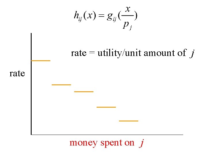
rate = utility/unit amount of j rate amount of j money spent on j

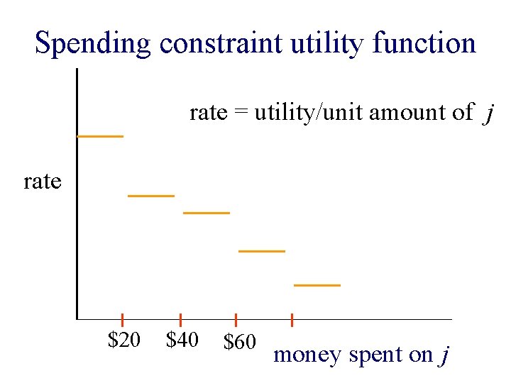
Spending constraint utility function rate = utility/unit amount of j rate $20 $40 $60 money spent on j

Spending constraint utility function n Happiness derived is not a function of allocation only but also of amount of money spent.

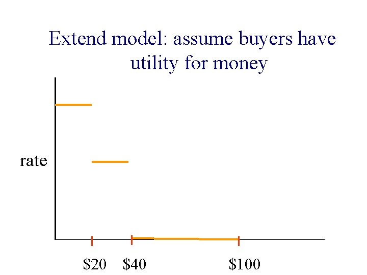
Extend model: assume buyers have utility for money rate $20 $40 $100

Theorem: Polynomial time algorithm for computing equilibrium prices and allocations for Fisher’s model with spending constraint utilities. Furthermore, equilibrium prices are unique.

Satisfies weak gross substitutability!

Old pieces become more complex + there are new pieces

But they still fit just right!

Don Patinkin, 1956 n Money, Interest, and Prices. An Integration of Monetary and Value Theory n Pascal Bridel, 2002: ¨ Euro. J. History of Economic Thought, Patinkin, Walras and the ‘money-in-the-utilityfunction’ tradition

An unexpected fallout!!

An unexpected fallout!! n A new kind of utility function ¨ Happiness derived is not a function of allocation only but also of amount of money spent.

An unexpected fallout!! n A new kind of utility function ¨ Happiness derived is not a function of allocation only but also of amount of money spent. n Has applications in Google’s Ad. Words Market!

A digression

The view 5 years ago: Relevant Search Results

Business world’s view now : (as Advertisement companies)

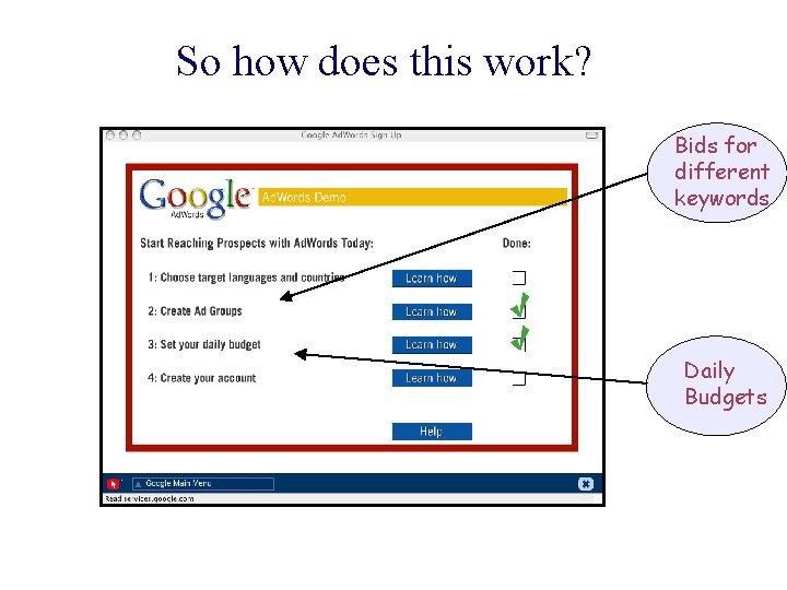
So how does this work? Bids for different keywords Daily Budgets

An interesting algorithmic question! n Monika Henzinger, 2004: Find an on-line algorithm that maximizes Google’s revenue.

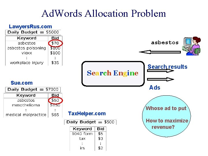
Ad. Words Allocation Problem Lawyers. Rus. com asbestos Search Engine Sue. com Search results Ads Tax. Helper. com Whose ad to put How to maximize revenue?

Ad. Words Problem n Mehta, Saberi, Vazirani & Vazirani, 2005: 1 -1/e algorithm, assuming budgets>>bids

Ad. Words Problem n Mehta, Saberi, Vazirani & Vazirani, 2005: 1 -1/e algorithm, assuming budgets>>bids Optimal!

Ad. Words Problem n Mehta, Saberi, Vazirani & Vazirani, 2005: 1 -1/e algorithm, assuming budgets>>bids Optimal!

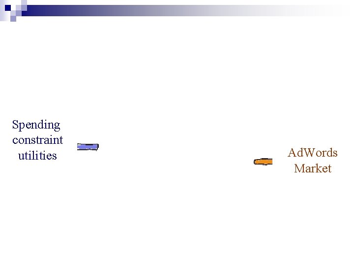
Spending constraint utilities Ad. Words Market

Ad. Words market n Assume that Google will determine equilibrium price/click for keywords

Ad. Words market n Assume that Google will determine equilibrium price/click for keywords n How should advertisers specify their utility functions?

Choice of utility function n Expressive enough that advertisers get close to their ‘‘optimal’’ allocations

Choice of utility function n Expressive enough that advertisers get close to their ‘‘optimal’’ allocations n Efficiently computable

Choice of utility function n Expressive enough that advertisers get close to their ‘‘optimal’’ allocations n Efficiently computable n Easy to specify utilities

n linear utility function: a business will typically get only one type of query throughout the day!

n linear utility function: a business will typically get only one type of query throughout the day! n concave utility function: no efficient algorithm known!

n linear utility function: a business will typically get only one type of query throughout the day! n concave utility function: no efficient algorithm known! ¨ Difficult for advertisers to define concave functions

Easier for a buyer n To say how much money she should spend on each good, for a range of prices, rather than how happy she is with a given bundle.

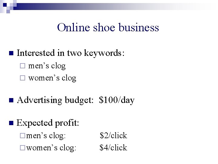
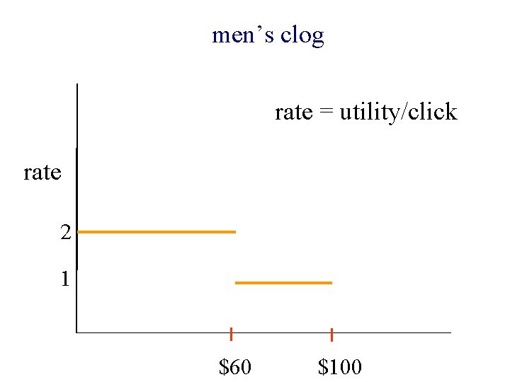
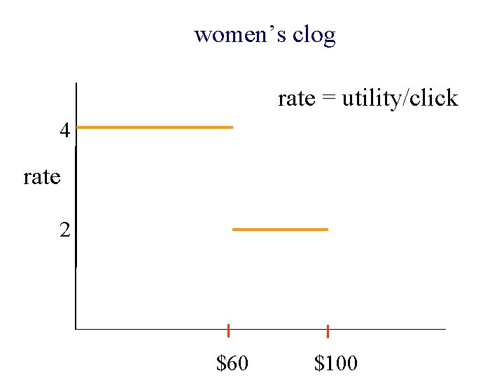
Online shoe business n Interested in two keywords: men’s clog ¨ women’s clog ¨ n Advertising budget: $100/day n Expected profit: ¨ men’s clog: ¨ women’s clog: $2/click $4/click

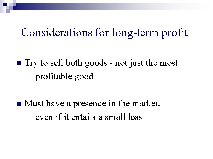
Considerations for long-term profit n Try to sell both goods - not just the most profitable good n Must have a presence in the market, even if it entails a small loss

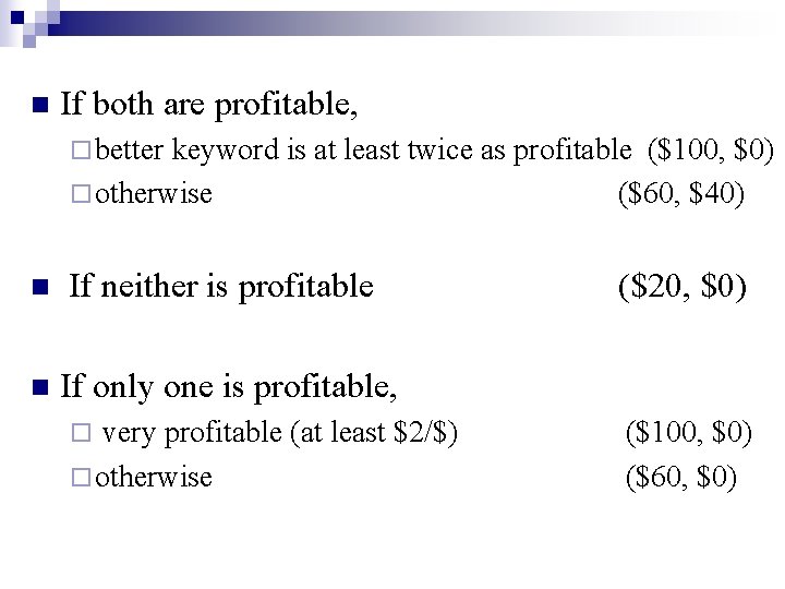
n If both are profitable, ¨ better keyword is at least twice as profitable ($100, $0) ¨ otherwise ($60, $40) n If neither is profitable n If only one is profitable, very profitable (at least $2/$) ¨ otherwise ¨ ($20, $0) ($100, $0) ($60, $0)

men’s clog rate = utility/click rate 2 1 $60 $100

women’s clog rate = utility/click 4 rate 2 $60 $100

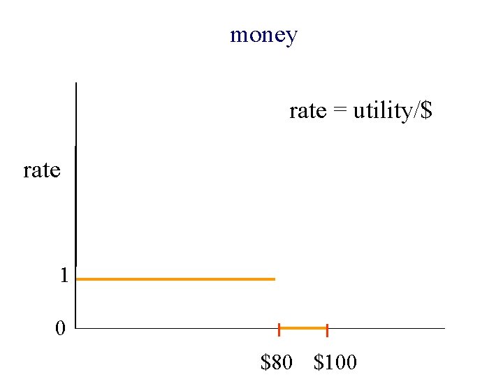
money rate = utility/$ rate 1 0 $80 $100

Ad. Words market n Suppose Google stays with auctions but allows advertisers to specify bids in the spending constraint model

Ad. Words market n Suppose Google stays with auctions but allows advertisers to specify bids in the spending constraint model ¨ expressivity!

Ad. Words market n Suppose Google stays with auctions but allows advertisers to specify bids in the spending constraint model ¨ expressivity! n Good online algorithm for maximizing Google’s revenues?

n Goel & Mehta, 2006: A small modification to the MSVV algorithm achieves 1 – 1/e competitive ratio!

Open Is there a convex program that captures equilibrium allocations for spending constraint utilities?

Spending constraint utilities satisfy n Equilibrium exists (under mild conditions) n Equilibrium utilities and prices are unique n Rational n With small denominators

Linear utilities also satisfy n Equilibrium exists (under mild conditions) n Equilibrium utilities and prices are unique n Rational n With small denominators

Proof follows from Eisenberg-Gale Convex Program, 1959

For spending constraint utilities, proof follows from algorithm, and not a convex program!

Open Is there an LP whose optimal solutions capture equilibrium allocations for Fisher’s linear case?

Open Use spending constraint algorithm to solve piecewise linear, concave utilities

Algorithms & Game Theory common origins von Neumann, 1928: minimax theorem for 2 -person zero sum games n von Neumann & Morgenstern, 1944: Games and Economic Behavior n von Neumann, 1946: Report on EDVAC n n Dantzig, Gale, Kuhn, Scarf, Tucker …

Piece-wise linear, concave utility amount of j

Differentiate rate = utility/unit amount of j rate amount of j

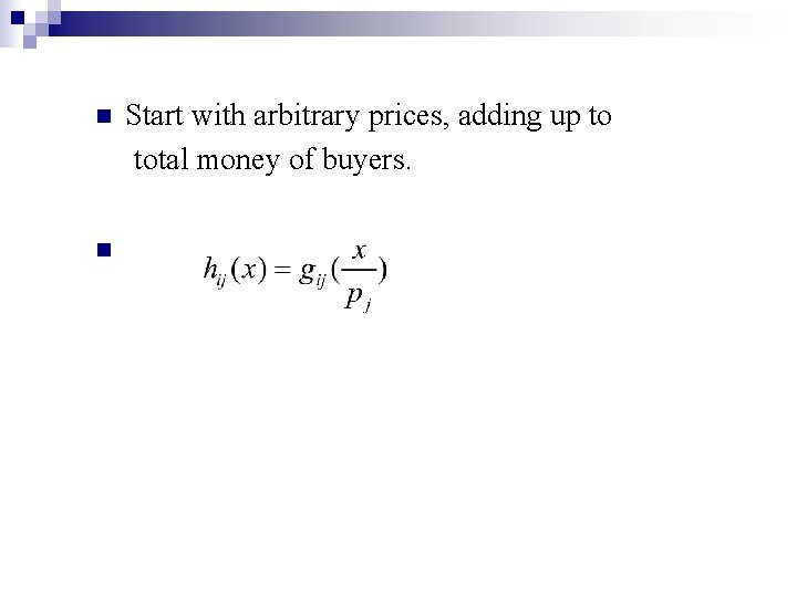
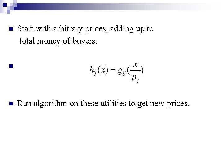
n n Start with arbitrary prices, adding up to total money of buyers.

rate = utility/unit amount of j rate money spent on j

n Start with arbitrary prices, adding up to total money of buyers. n n Run algorithm on these utilities to get new prices.

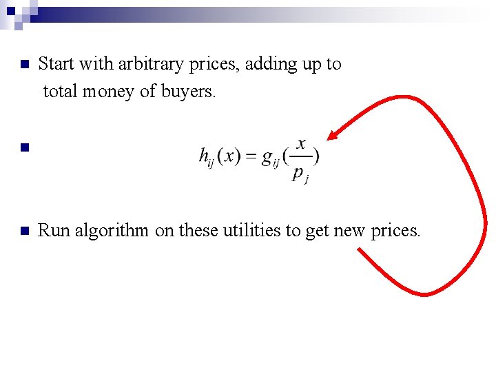
n Start with arbitrary prices, adding up to total money of buyers. n n Run algorithm on these utilities to get new prices.

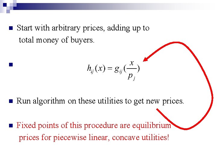
n Start with arbitrary prices, adding up to total money of buyers. n n Run algorithm on these utilities to get new prices. n Fixed points of this procedure are equilibrium prices for piecewise linear, concave utilities!