New Market Models Algorithmic Game Theory and Algorithms

New Market Models Algorithmic Game Theory and Algorithms and Internet Computing Vijay V. Vazirani Georgia Tech

Algorithmic ratification of the “invisible hand of the market” How do we salvage the situation? ?

What is the “right” model? ?

Linear Fisher Market n DPSV, 2002: First polynomial time algorithm n Extend to separable, plc utilities? ?

What makes linear utilities easy? n Weak gross substitutability: Increasing price of one good cannot decrease demand of another. n Piecewise-linear, concave utilities do not satisfy this.

Piecewise linear, concave utility amount of j

Differentiate rate = utility/unit amount of j rate amount of j

rate = utility/unit amount of j rate amount of j money spent on j

Spending constraint utility function rate = utility/unit amount of j rate $20 $40 $60 money spent on j

n Theorem (V. , 2002): Spending constraint utilities: 1). Satisfy weak gross substitutability 2). Polynomial time algorithm for computing equilibrium 3). Equilibrium is rational.

An unexpected fallout!! n Has applications to Google’s Ad. Words Market!

Application to Adwords market rate = utility/click rate $20 $40 $60 money spent on keyword j

Is there a convex program for this model? n “We believe the answer to this question should be ‘yes’. In our experience, non-trivial polynomial time algorithms for problems are rare and happen for a good reason – a deep mathematical structure intimately connected to the problem. ”

Devanur’s program for linear Fisher

C. P. for spending constraint!

Spending constraint market Fisher market with plc utilities EG convex program = Devanur’s program

Price discrimination markets n Business charges different prices from different customers for essentially same goods or services. Goel & V. , 2009: Perfect price discrimination market. Business charges each consumer what they are willing and able to pay. n

plc utilities

n Middleman buys all goods and sells to buyers, charging according to utility accrued. n Given p, each buyer picks rate for accruing utility.

n Middleman buys all goods and sells to buyers, charging according to utility accrued. n Given p, each buyer picks rate for accruing utility. n Equilibrium is captured by a rational convex program!

Generalization of EG program works!

V. , 2010: Generalize to n Continuously differentiable, quasiconcave (non-separable) utilities, satisfying non-satiation.

V. , 2010: Generalize to n Continuously differentiable, quasiconcave (non-separable) utilities, satisfying non-satiation. Compare with Arrow-Debreu utilities!! continuous, quasiconcave, satisfying non-satiation. n

Spending constraint market Price discrimination market (plc utilities) EG convex program = Devanur’s program

Eisenberg-Gale Markets Jain & V. , 2007 Price disc. market (Proportional Fairness) (Kelly, 1997) Nash Bargaining V. , 2008 EG convex program = Spending constraint market Devanur’s program

A combinatorial market

A combinatorial market

A combinatorial market

A combinatorial market n Given: ¨ Network G = (V, E) (directed or undirected) ¨ Capacities on edges c(e) ¨ Agents: source-sink pairs with money m(1), … m(k) n Find: equilibrium flows and edge prices

Equilibrium n Flows and edge prices f(i): flow of agent i ¨ p(e): price/unit flow of edge e ¨ n Satisfying: p(e)>0 only if e is saturated ¨ flows go on cheapest paths ¨ money of each agent is fully spent ¨

Kelly’s resource allocation model, 1997 Mathematical framework for understanding TCP congestion control

n Van Jacobson, 1988: AIMD protocol (Additive Increase Multiplicative Decrease)

n Van Jacobson, 1988: AIMD protocol (Additive Increase Multiplicative Decrease) n Why does it work so well?

n Van Jacobson, 1988: AIMD protocol (Additive Increase Multiplicative Decrease) n Why does it work so well? n Kelly, 1977: Highly successful theory

TCP Congestion Control f(i): source rate n p(e): prob. of packet loss (in TCP Reno) queueing delay (in TCP Vegas) n

TCP Congestion Control n n n f(i): source rate p(e): prob. of packet loss (in TCP Reno) queueing delay (in TCP Vegas) Low & Lapsley, 1999: AIMD + RED converges to equilibrium in limit

TCP Congestion Control n n f(i): source rate p(e): prob. of packet loss (in TCP Reno) queueing delay (in TCP Vegas) Kelly: Equilibrium flows are proportionally fair: only way of adding 5% flow to someone is to decrease total of 5% flow from rest.

n Kelly & V. , 2002: Kelly’s model is a generalization of Fisher’s model.

n Kelly & V. , 2002: Kelly’s model is a generalization of Fisher’s model. n Find combinatorial poly time algorithms!

n Kelly & V. , 2002: Kelly’s model is a generalization of Fisher’s model. n Find combinatorial poly time algorithms! (May lead to new insights for TCP congestion control protocol)

Jain & V. , 2005: n Strongly polynomial combinatorial algorithm for single-source multiple-sink market

Single-source multiple-sink market n Given: ¨ Network G = (V, E), s: source ¨ Capacities on edges c(e) ¨ Agents: sinks with money n Find: equilibrium flows and edge prices

Equilibrium n Flows and edge prices f(i): flow of agent i ¨ p(e): price/unit flow of edge e ¨ n Satisfying: p(e)>0 only if e is saturated ¨ flows go on cheapest paths ¨ money of each agent is fully spent ¨

$5 $5

$30 $10 $40

Jain & V. , 2005: n Strongly polynomial combinatorial algorithm for single-source multiple-sink market n Ascending price auction ¨ Buyers: sinks (fixed budgets, maximize flow) ¨ Sellers: edges (maximize price)

Auction of k identical goods p = 0; n while there are >k buyers: raise p; n end; n sell to remaining k buyers at price p; n

Find equilibrium prices and flows

Find equilibrium prices and flows cap(e)

60 min-cut separating from all the sinks

60

60

Throughout the algorithm: c(i): cost of cheapest path from sink demands flow to

sink 60 demands flow

Auction of edges in cut p = 0; n while the cut is over-saturated: raise p; n end; n assign price p to all edges in the cut; n

60 50

60 50

60 50 20

60 50 20

60 50 20

60 50 20 nested cuts

n Flow and prices will: ¨ Saturate all red cuts ¨ Use up sinks’ money ¨ Send flow on cheapest paths

n Exercise: Find the red cuts efficiently!

Convex Program for Kelly’s Model

JV Algorithm n primal-dual alg. for nonlinear convex program n “primal” variables: flows n “dual” variables: prices of edges n algorithm: primal & dual improvements Allocations Prices

Rational!!

Other resource allocation markets n k source-sink pairs (directed/undirected)

Other resource allocation markets k source-sink pairs (directed/undirected) n Branchings rooted at sources (agents) n Spanning trees n Network coding n

Branching market (for broadcasting)

Branching market (for broadcasting)

Branching market (for broadcasting)

Branching market (for broadcasting)

Branching market (for broadcasting) n Given: Network G = (V, E), directed ¨ edge capacities ¨ sources, ¨ money of each source n Find: edge prices and a packing of branchings rooted at sources s. t. p(e) > 0 => e is saturated ¨ each branching is cheapest possible ¨ money of each source fully used. ¨

Eisenberg-Gale-type program for branching market s. t. packing of branchings

Eisenberg-Gale-Type Convex Program s. t. packing constraints

Eisenberg-Gale Market n A market whose equilibrium is captured as an optimal solution to an Eisenberg-Gale-type program

Other resource allocation markets k source-sink pairs (directed/undirected) n Branchings rooted at sources (agents) n Spanning trees n Network coding n

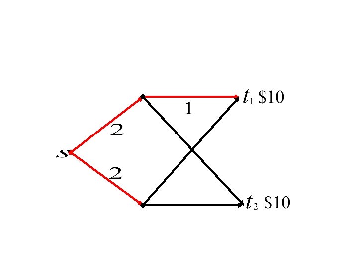
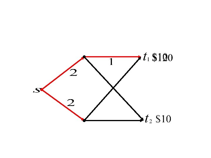
Irrational for 2 sources & 3 sinks $1 $1 $1

Irrational for 2 sources & 3 sinks Equilibrium prices

Max-flow min-cut theorem!

n Theorem: Strongly polynomial algs for following markets : ¨ 2 source-sink pairs, undirected (Hu, 1963) ¨ spanning tree (Nash-William & Tutte, 1961) ¨ 2 sources branching (Edmonds, 1967 + JV, 2005) n 3 sources branching: irrational

n Theorem: Strongly polynomial algs for following markets : ¨ 2 source-sink pairs, undirected (Hu, 1963) ¨ spanning tree (Nash-William & Tutte, 1961) ¨ 2 sources branching (Edmonds, 1967 + JV, 2005) n 3 sources branching: irrational n Open: (no max-min theorems): ¨ 2 source-sink pairs, directed ¨ 2 sources, network coding

Chakrabarty, Devanur & V. , 2006: n EG[2]: Eisenberg-Gale markets with 2 agents n Theorem: EG[2] markets are rational.

Chakrabarty, Devanur & V. , 2006: n EG[2]: Eisenberg-Gale markets with 2 agents n Theorem: EG[2] markets are rational. n Combinatorial EG[2] markets: polytope of feasible utilities can be described via combinatorial LP. n Theorem: Strongly poly alg for Comb EG[2].

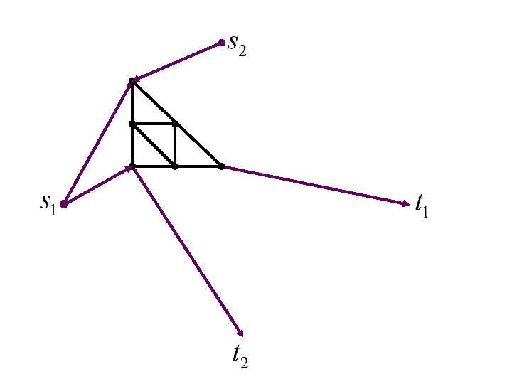
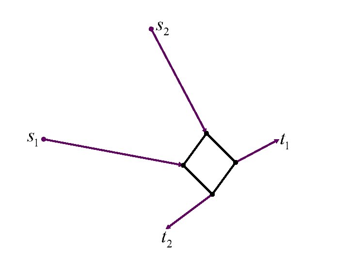
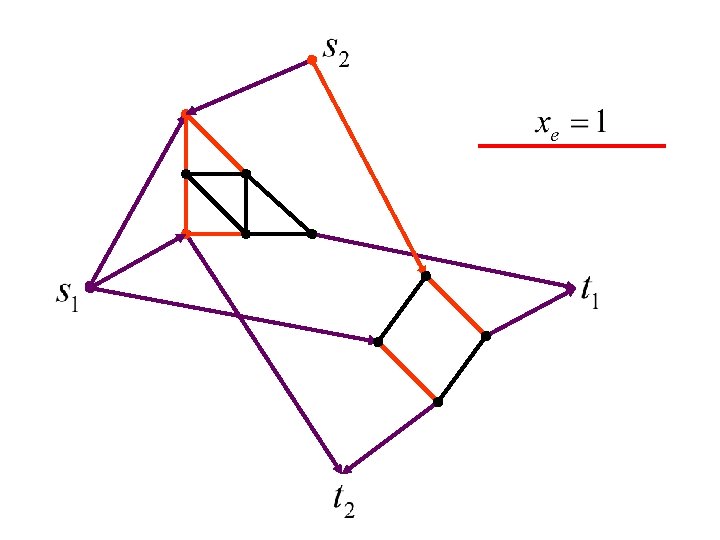
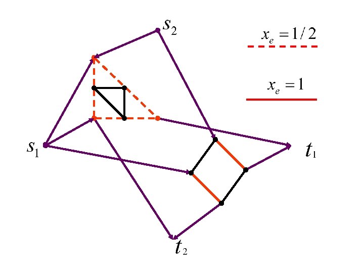
2 source-sink market in directed graphs

2 1

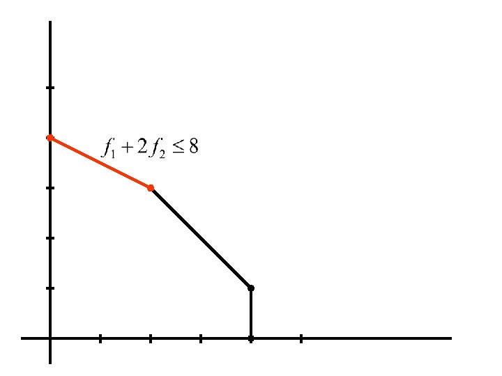
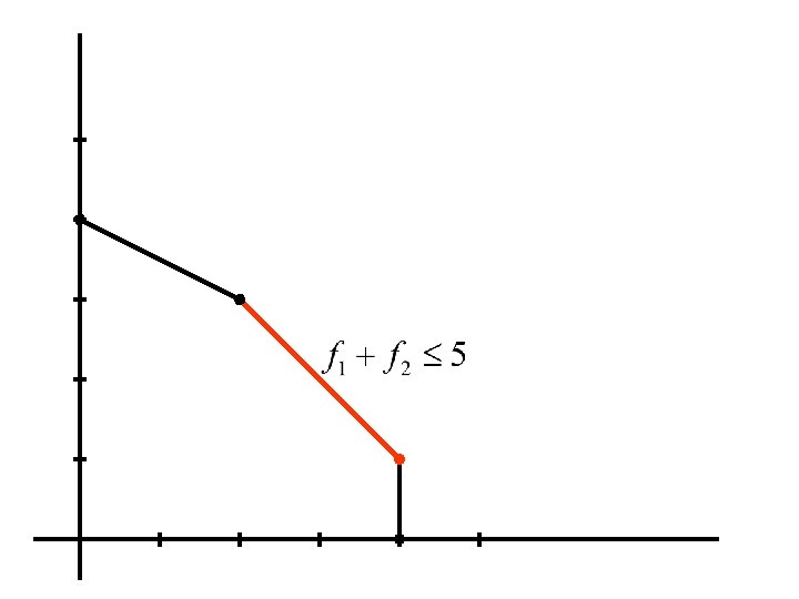
Polytope of feasible flows

LP’s corresponding to facets

$30 $60

Polytope of feasible flows 2 (1, 2) 1 (0, 1) 0

n Find the two (one) facets n Exponentially many facets! n Binary search on

$5 $10

n Find relative ‘‘prices’’ of two facets, say n Compute duals

n Find relative ‘‘prices’’ of two facets, say n Compute duals n Compute

$5, each

10/2 = $5, each $10, each

$10 $5 $30 $15 $60

$10 $5 $30 $15 $60

$10 $5 $30=$15 x 2 $15 $60=$20 x 3

3 -source branching Single-source 2 s-s undir SUA Comb EG[2] 2 s-s dir Fisher EG[2] EG Rational