Introduction to Algorithmic Trading Strategies Lecture 7 Portfolio

Introduction to Algorithmic Trading Strategies Lecture 7 Portfolio Optimization Haksun Li haksun. li@numericalmethod. com www. numericalmethod. com

Outline � Sharpe Ratio � Problems with Sharpe Ratio � Omega � Properties of Omega � Portfolio Optimization

References � Connor Keating, William Shadwick. A universal performance measure. Finance and Investment Conference 2002. 26 June 2002. � Connor Keating, William Shadwick. An introduction to Omega. 2002. � Kazemi, Scheeweis and Gupta. Omega as a performance measure. 2003. � S. Avouyi-Dovi, A. Morin, and D. Neto. Optimal asset allocation with Omega function. Tech. report, Banque de France, 2004. Research Paper.

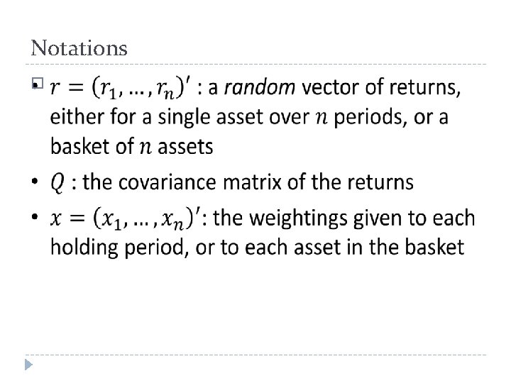
Notations �

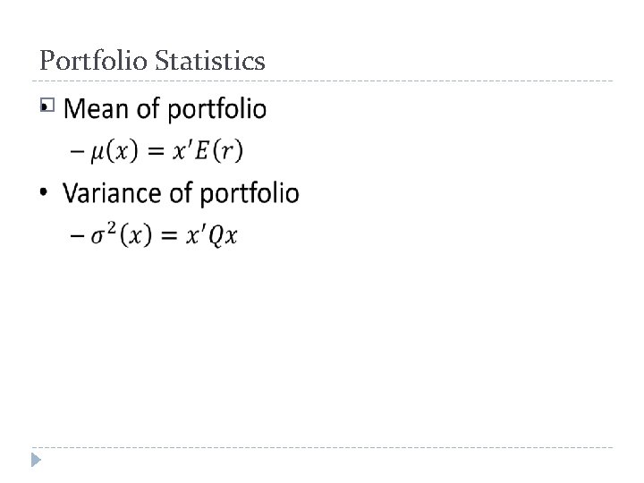
Portfolio Statistics �

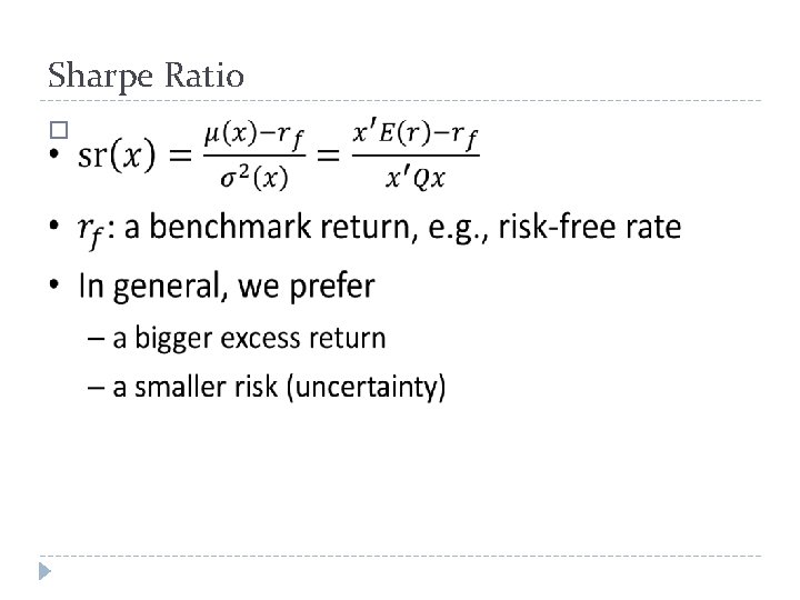
Sharpe Ratio �

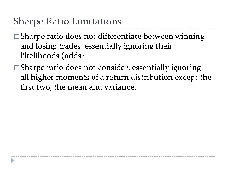
Sharpe Ratio Limitations � Sharpe ratio does not differentiate between winning and losing trades, essentially ignoring their likelihoods (odds). � Sharpe ratio does not consider, essentially ignoring, all higher moments of a return distribution except the first two, the mean and variance.

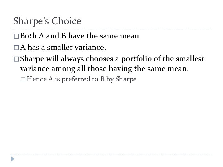
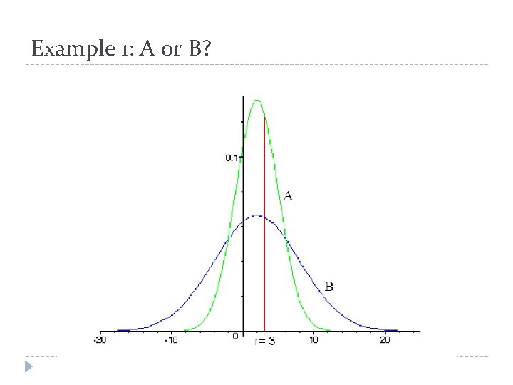
Sharpe’s Choice � Both A and B have the same mean. � A has a smaller variance. � Sharpe will always chooses a portfolio of the smallest variance among all those having the same mean. � Hence A is preferred to B by Sharpe.

Avoid Downsides and Upsides � Sharpe chooses the smallest variance portfolio to reduce the chance of having extreme losses. � Yet, for a Normally distributed return, the extreme gains are as likely as the extreme losses. � Ignoring the downsides will inevitably ignore the potential for upsides as well.

Potential for Gains � Suppose we rank A and B by their potential for gains, we would choose B over A. � Shall we choose the portfolio with the biggest variance then? � It is very counter intuitive.

Example 1: A or B?

Example 1: L = 3 � Suppose the loss threshold is 3. � Pictorially, we see that B has more mass to the right of 3 than that of A. � B: 43% of mass; A: 37%. � We compare the likelihood of winning to losing. � B: 0. 77; A: 0. 59. � We therefore prefer B to A.

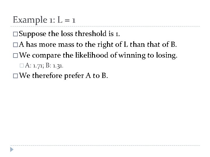
Example 1: L = 1 � Suppose the loss threshold is 1. � A has more mass to the right of L than that of B. � We compare the likelihood of winning to losing. � A: 1. 71; B: 1. 31. � We therefore prefer A to B.

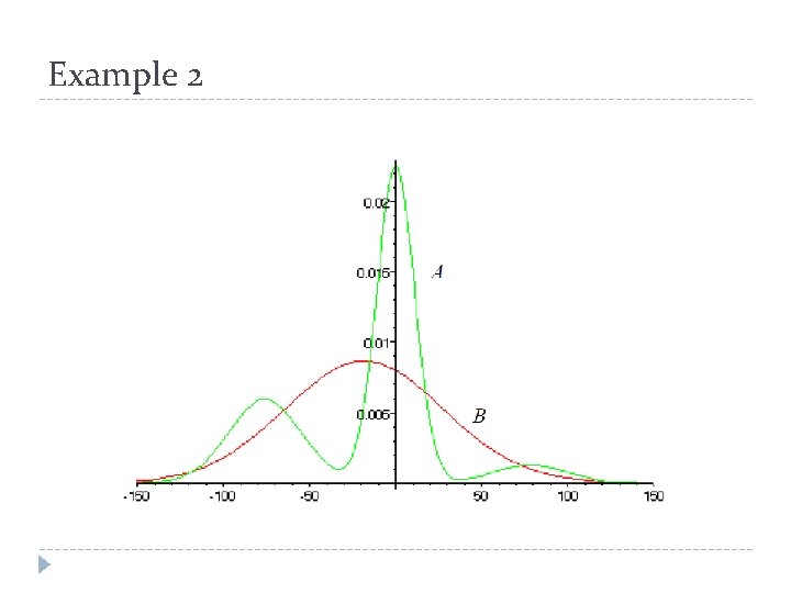
Example 2

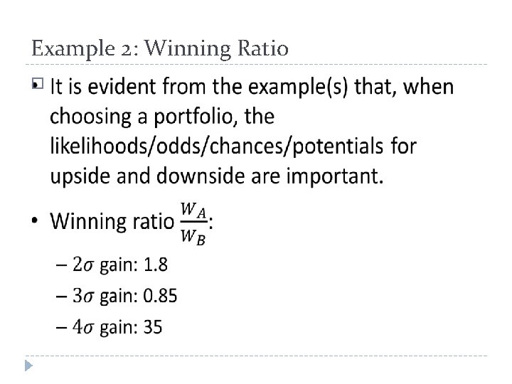
Example 2: Winning Ratio �

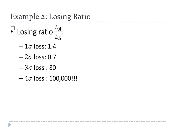
Example 2: Losing Ratio �

Higher Moments Are Important � Both large gains and losses in example 2 are produced by moments of order 5 and higher. � They even shadow the effects of skew and kurtosis. � Example 2 has the same mean and variance for both distributions. � Because Sharpe Ratio ignores all moments from order 3 and bigger, it treats all these very different distributions the same.

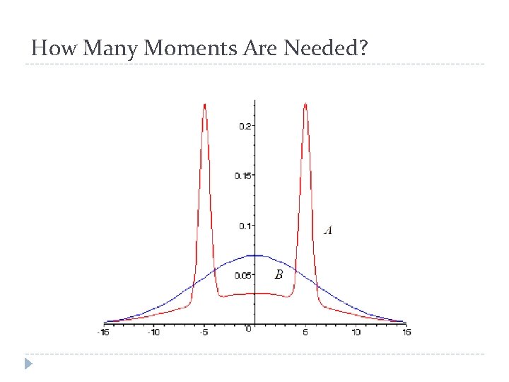
How Many Moments Are Needed?

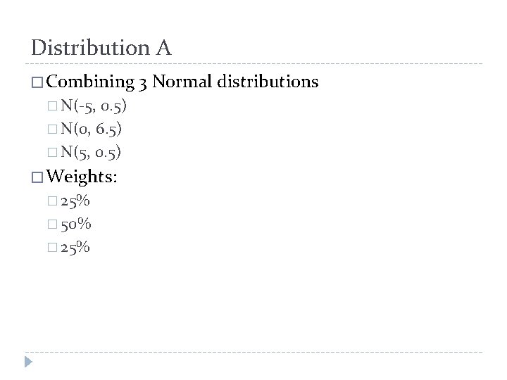
Distribution A � Combining 3 Normal distributions � N(-5, 0. 5) � N(0, 6. 5) � N(5, 0. 5) � Weights: � 25% � 50% � 25%

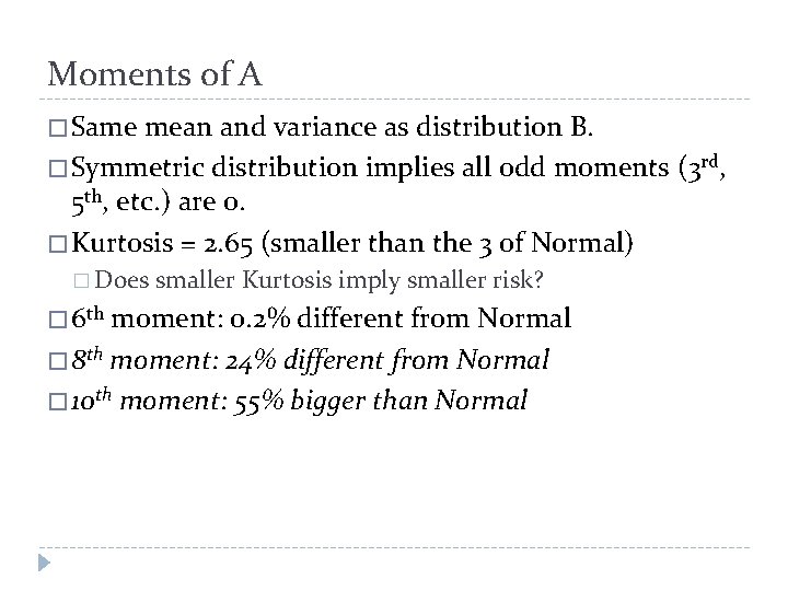
Moments of A � Same mean and variance as distribution B. � Symmetric distribution implies all odd moments (3 rd, 5 th, etc. ) are 0. � Kurtosis = 2. 65 (smaller than the 3 of Normal) � Does smaller Kurtosis imply smaller risk? � 6 th moment: 0. 2% different from Normal � 8 th moment: 24% different from Normal � 10 th moment: 55% bigger than Normal

Performance Measure Requirements � Take into account the odds of winning and losing. � Take into account the sizes of winning and losing. � Take into account of (all) the moments of a return distribution.

Loss Threshold � Clearly, the definition, hence likelihoods, of winning and losing depends on how we define loss. � Suppose L = Loss Threshold, � for return < L, we consider it a loss � for return > L, we consider it a gain

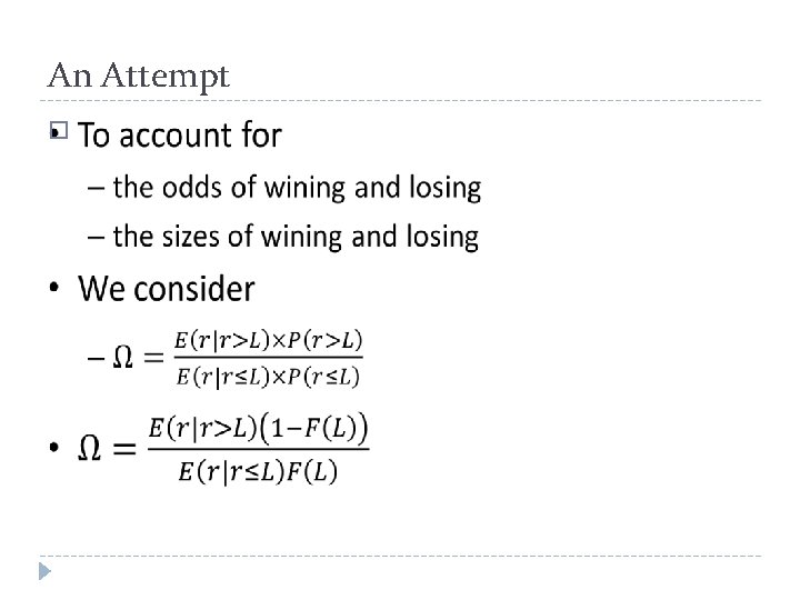
An Attempt �

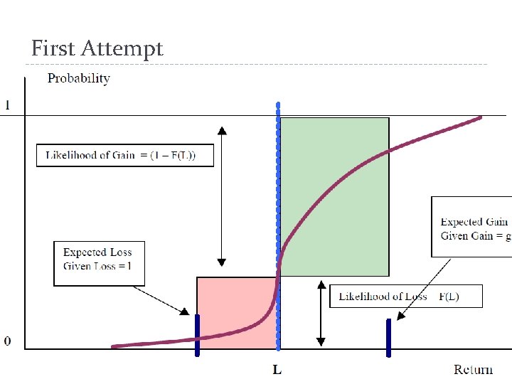
First Attempt

First Attempt Inadequacy � Why F(L)? � Not using the information from the entire distribution. � hence ignoring higher moments

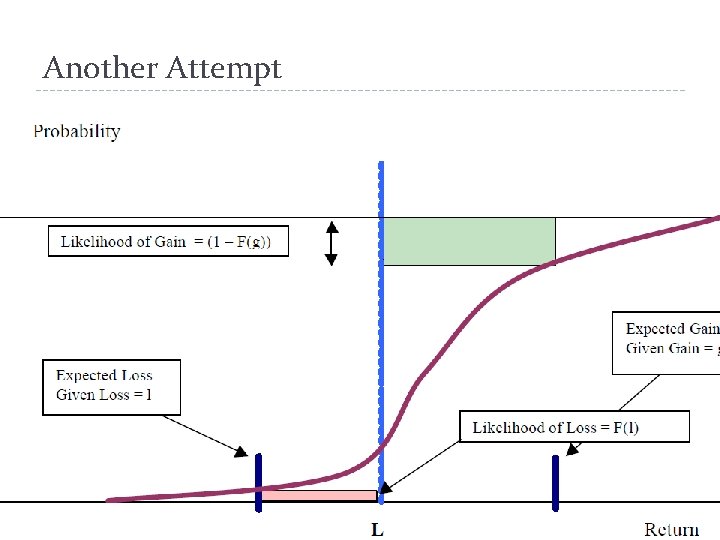
Another Attempt

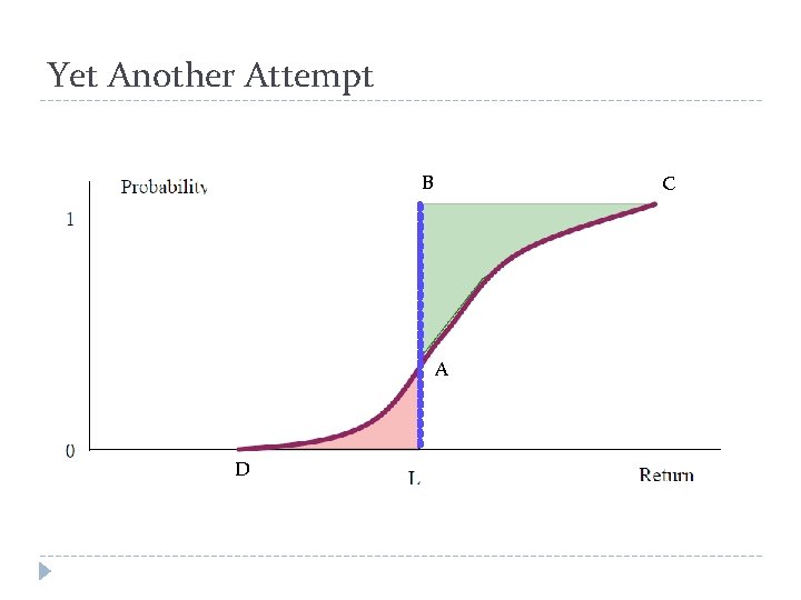
Yet Another Attempt B C A D

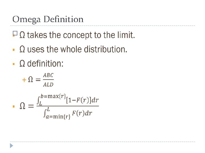
Omega Definition �

Intuitions � Omega is a ratio of winning size weighted by probabilities to losing size weighted by probabilities. � Omega considers size and odds of winning and losing trades. � Omega considers all moments because the definition incorporates the whole distribution.

Omega Advantages � There is no parameter (estimation). � There is no need to estimate (higher) moments. � Work with all kinds of distributions. � Use a function (of Loss Threshold) to measure performance rather than a single number (as in Sharpe Ratio). � It is as smooth as the return distribution. � It is monotonic decreasing.

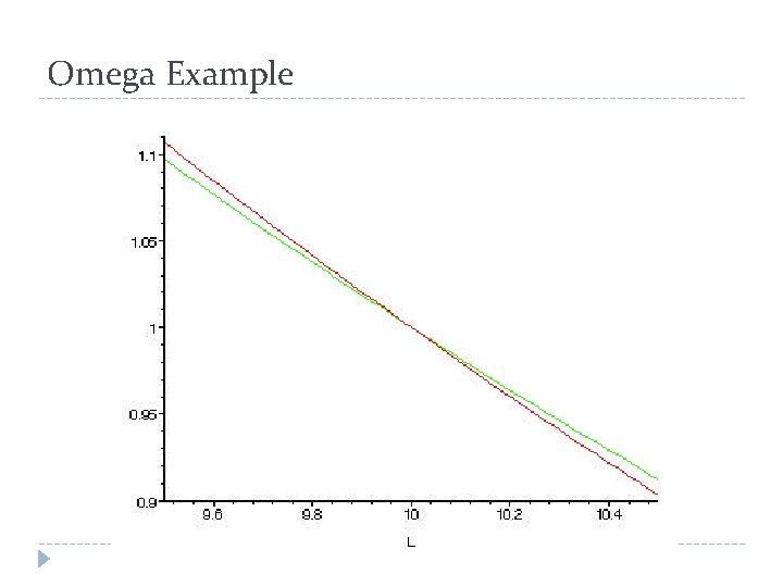
Omega Example

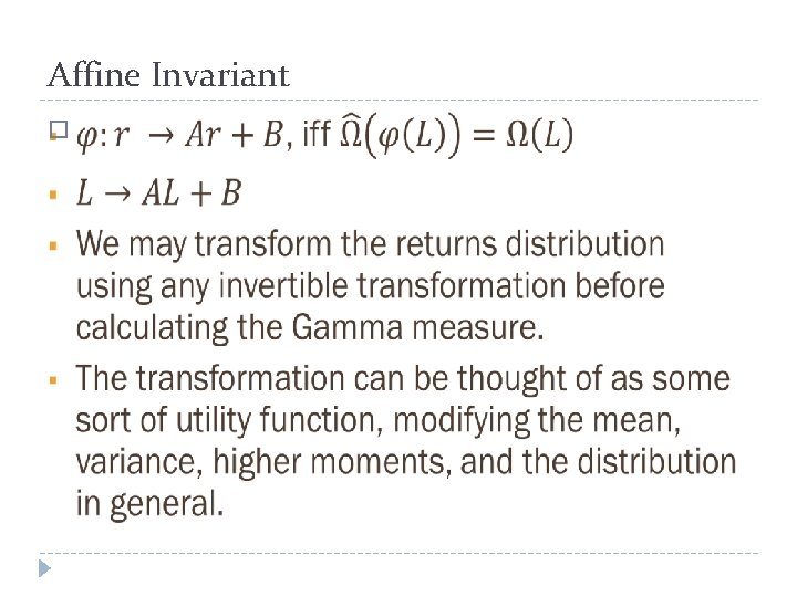
Affine Invariant �

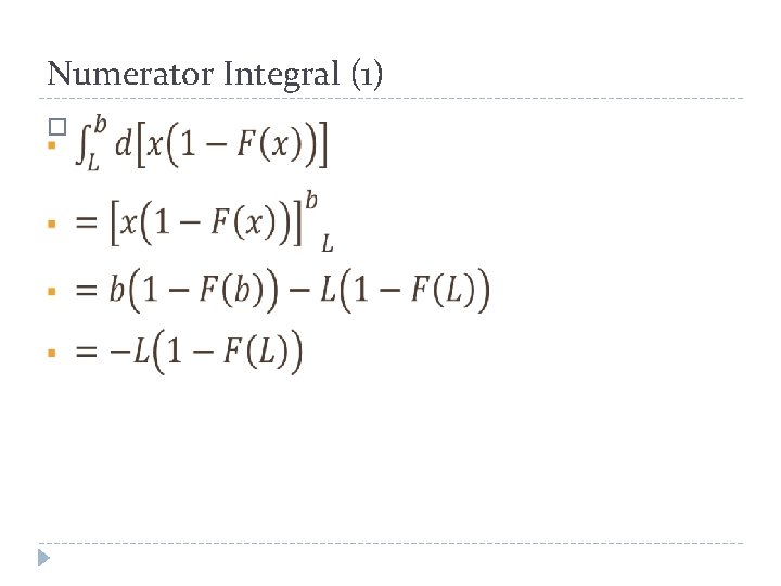
Numerator Integral (1) �

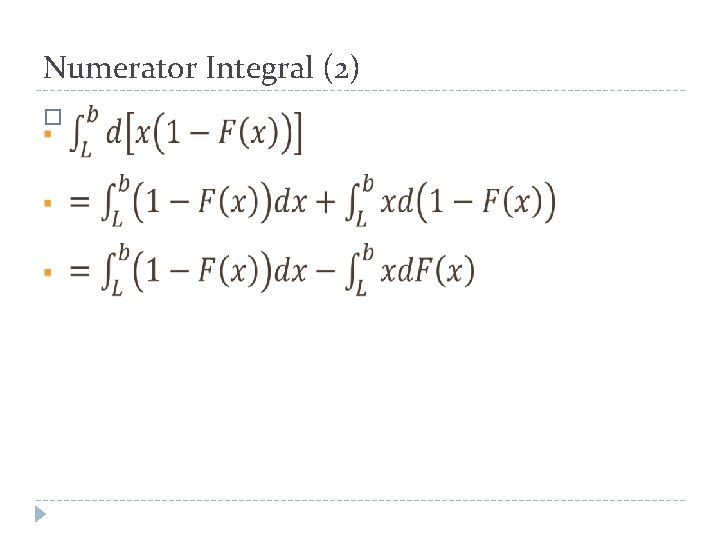
Numerator Integral (2) �

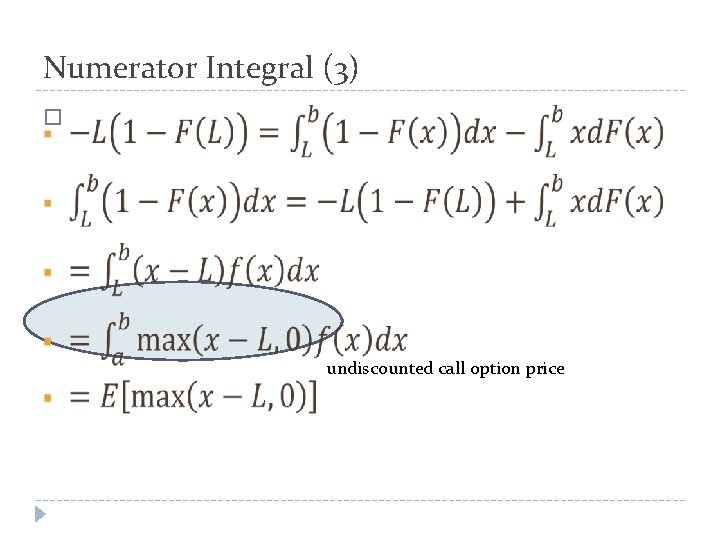
Numerator Integral (3) � undiscounted call option price

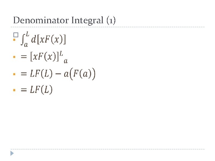
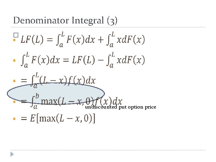
Denominator Integral (1) �

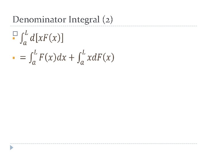
Denominator Integral (2) �

Denominator Integral (3) � undiscounted put option price

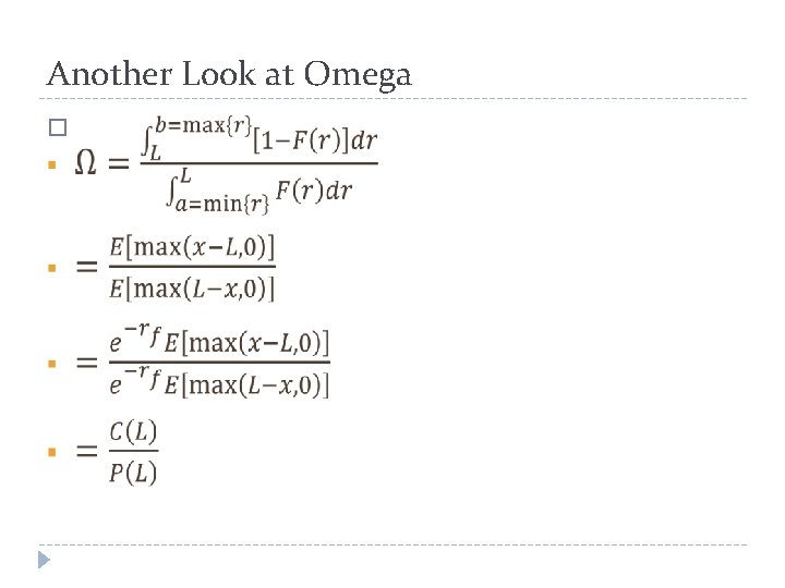
Another Look at Omega �

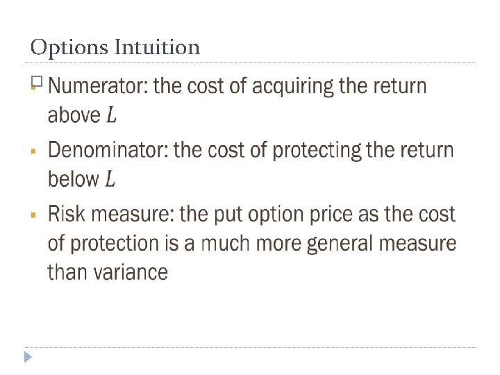
Options Intuition �

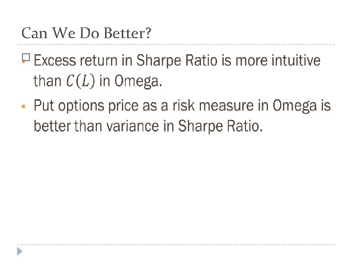
Can We Do Better? �

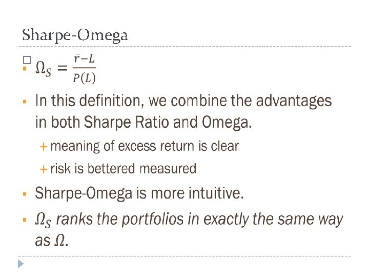
Sharpe-Omega �

Sharpe-Omega and Moments � It is important to note that the numerator relates only to the first moment (the mean) of the returns distribution. � It is the denominator that take into account the variance and all the higher moments, hence the whole distribution.

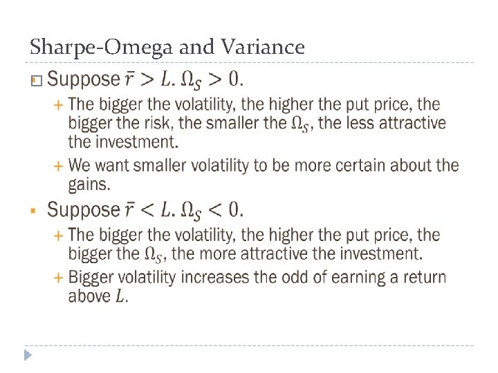
Sharpe-Omega and Variance �

Portfolio Optimization � In general, a Sharpe optimized portfolio is different from an Omega optimized portfolio.

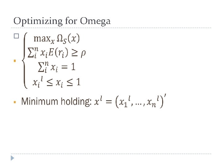
Optimizing for Omega �

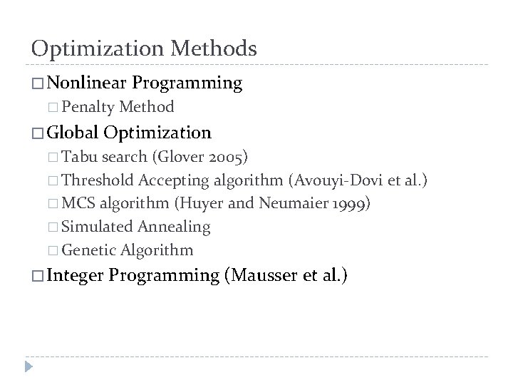
Optimization Methods � Nonlinear Programming � Penalty Method � Global Optimization � Tabu search (Glover 2005) � Threshold Accepting algorithm (Avouyi-Dovi et al. ) � MCS algorithm (Huyer and Neumaier 1999) � Simulated Annealing � Genetic Algorithm � Integer Programming (Mausser et al. )

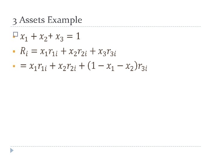
3 Assets Example �

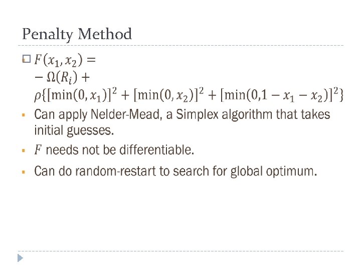
Penalty Method �

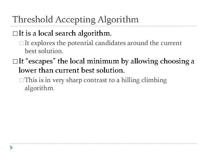
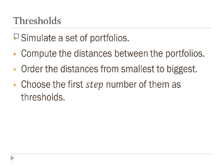
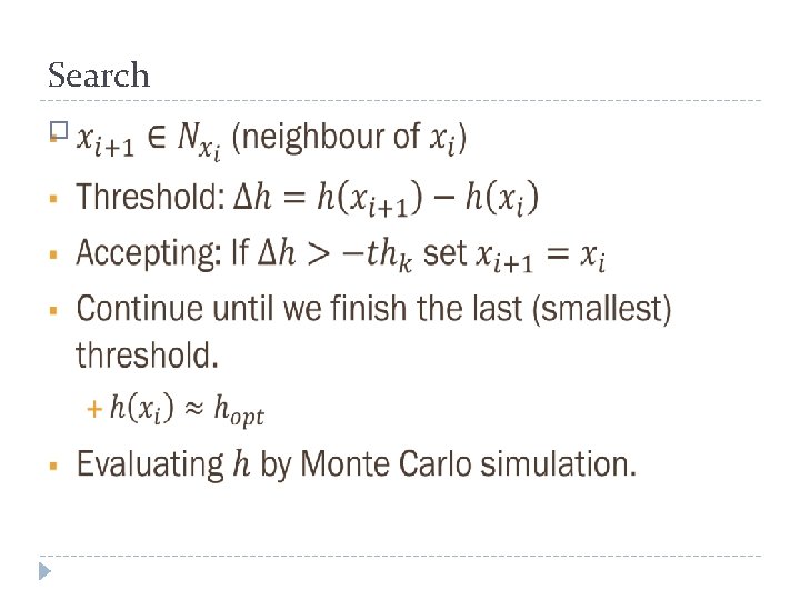
Threshold Accepting Algorithm � It is a local search algorithm. � It explores the potential candidates around the current best solution. � It “escapes” the local minimum by allowing choosing a lower than current best solution. � This is in very sharp contrast to a hilling climbing algorithm.

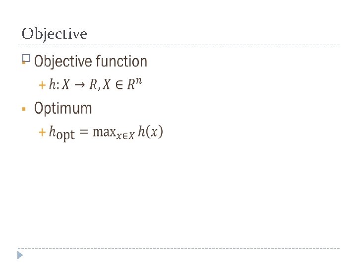
Objective �

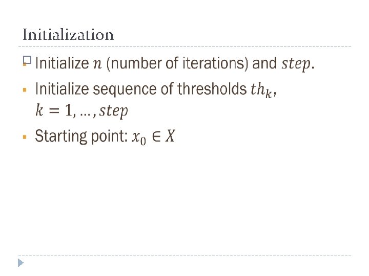
Initialization �

Thresholds �

Search �