Algorithmic and Algorithmic Game Theory Systems and Networked

Algorithmic and Algorithmic. Game. Theory Systems and. Networked Internet Computing Amin Saberi

Outline n Game Theory and Algorithms efficient algorithms for game theoretic notions n Complex networks and performance of basic algorithms

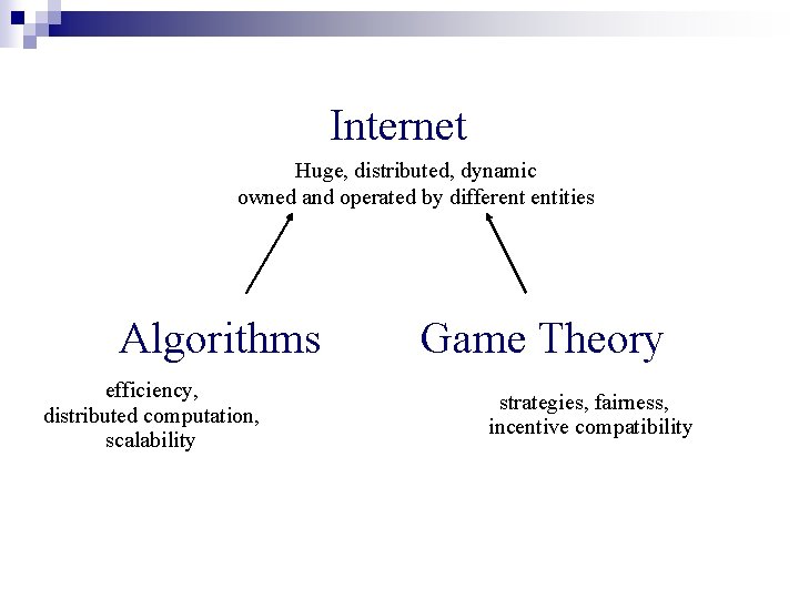
Internet Huge, distributed, dynamic owned and operated by different entities Algorithms efficiency, distributed computation, scalability Game Theory strategies, fairness, incentive compatibility

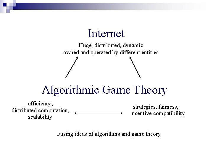
Internet Huge, distributed, dynamic owned and operated by different entities Algorithmic Game Theory efficiency, distributed computation, scalability strategies, fairness, incentive compatibility Fusing ideas of algorithms and game theory

Find efficient algorithms for computing game theoretic notions like: Market equilibria Nash equilibria Core Shapley value Auction. . .

Find efficient algorithms for computing game theoretic notions like: Market equilibria Nash equilibria Core Shapley value Auction. . .

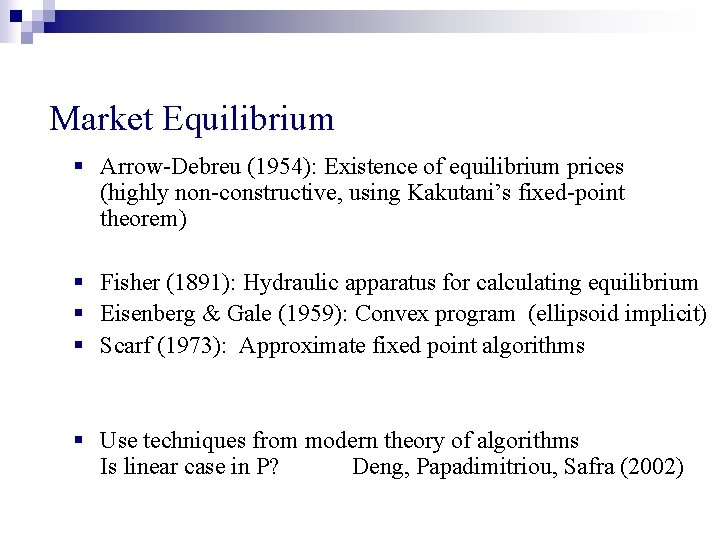
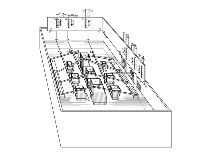
Market Equilibrium § Arrow-Debreu (1954): Existence of equilibrium prices (highly non-constructive, using Kakutani’s fixed-point theorem) § Fisher (1891): Hydraulic apparatus for calculating equilibrium § Eisenberg & Gale (1959): Convex program (ellipsoid implicit) § Scarf (1973): Approximate fixed point algorithms § Use techniques from modern theory of algorithms Is linear case in P? Deng, Papadimitriou, Safra (2002)

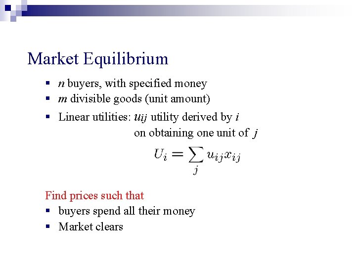
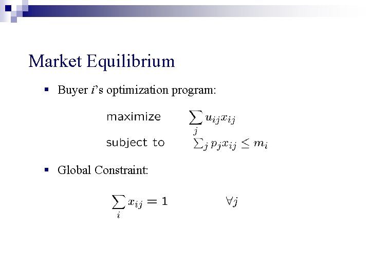
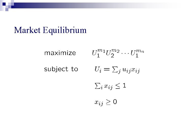
Market Equilibrium § n buyers, with specified money § m divisible goods (unit amount) § Linear utilities: uij utility derived by i on obtaining one unit of j Find prices such that § buyers spend all their money § Market clears

Market Equilibrium § Buyer i’s optimization program: § Global Constraint:

Market Equilibrium

Devanur, Papadimitriou, S. , Vazirani ‘ 03: A combinatorial (primal-dual) algorithm for finding the prices in polynomial time.

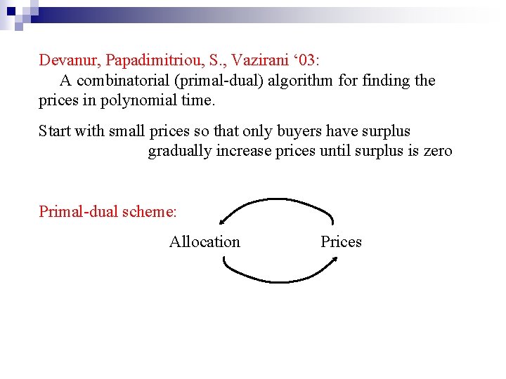
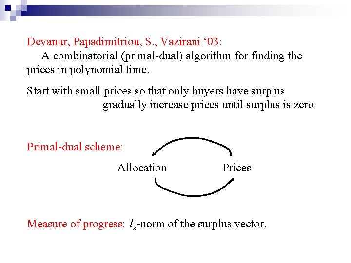
Devanur, Papadimitriou, S. , Vazirani ‘ 03: A combinatorial (primal-dual) algorithm for finding the prices in polynomial time. Start with small prices so that only buyers have surplus gradually increase prices until surplus is zero Primal-dual scheme: Allocation Prices

Devanur, Papadimitriou, S. , Vazirani ‘ 03: A combinatorial (primal-dual) algorithm for finding the prices in polynomial time. Start with small prices so that only buyers have surplus gradually increase prices until surplus is zero Primal-dual scheme: Allocation Prices Measure of progress: l 2 -norm of the surplus vector.

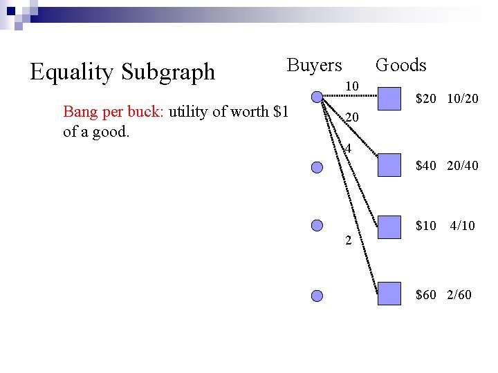
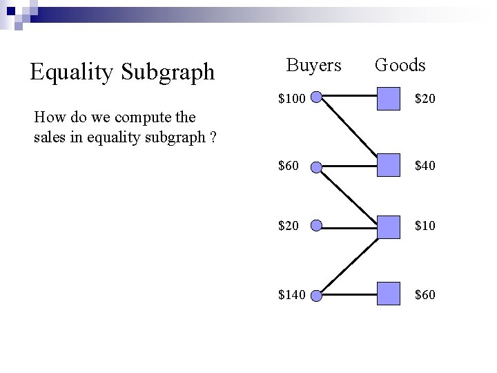
Equality Subgraph Buyers Bang per buck: utility of worth $1 of a good. Goods 10 $20 10/20 20 4 $40 20/40 2 $10 4/10 $60 2/60

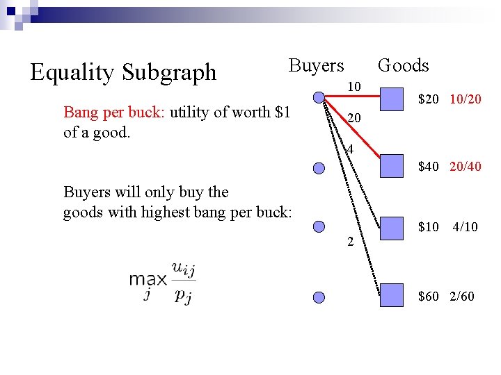
Equality Subgraph Buyers Bang per buck: utility of worth $1 of a good. Goods 10 $20 10/20 20 4 $40 20/40 Buyers will only buy the goods with highest bang per buck: 2 $10 4/10 $60 2/60

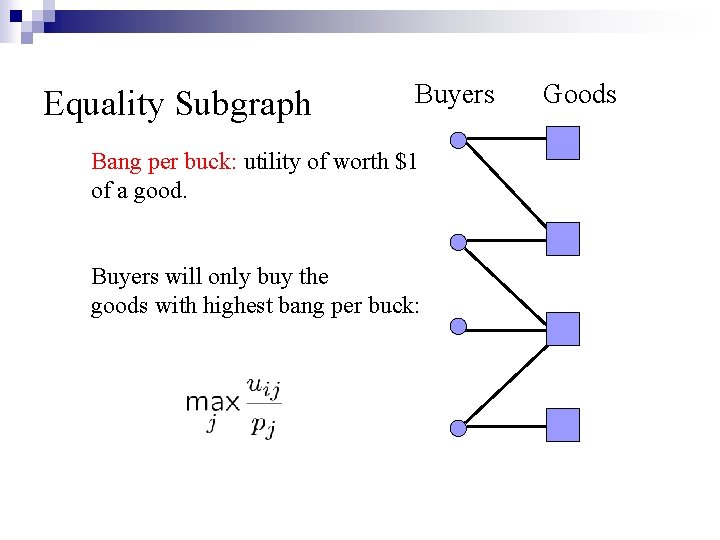
Equality Subgraph Buyers Bang per buck: utility of worth $1 of a good. Buyers will only buy the goods with highest bang per buck: Goods

Equality Subgraph Buyers Goods $100 $20 $60 $40 $20 $140 $60 How do we compute the sales in equality subgraph ?

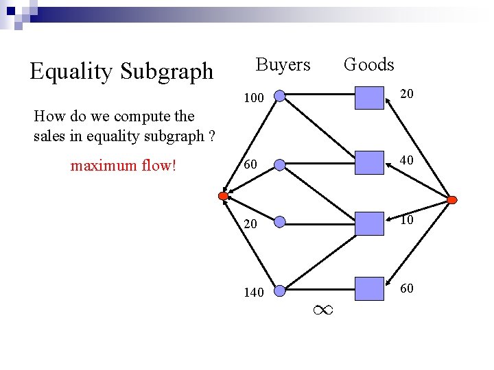
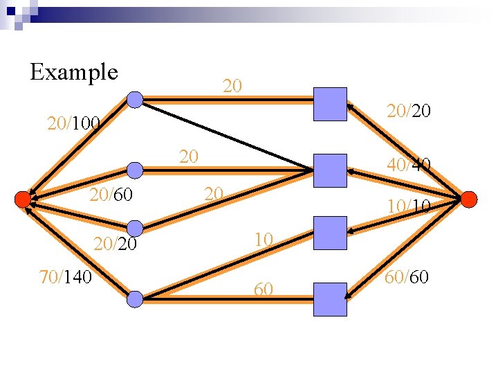
Equality Subgraph Buyers Goods 100 20 60 40 20 10 140 60 How do we compute the sales in equality subgraph ? maximum flow!

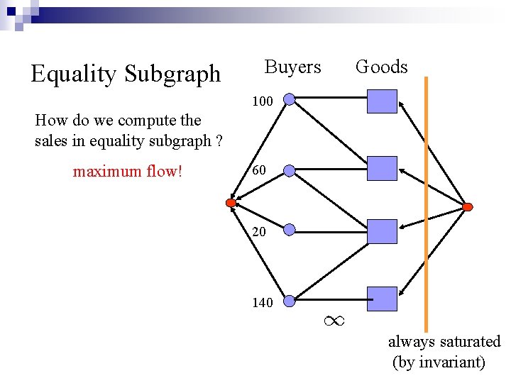
Equality Subgraph Buyers Goods 100 How do we compute the sales in equality subgraph ? maximum flow! 60 20 140 always saturated (by invariant)

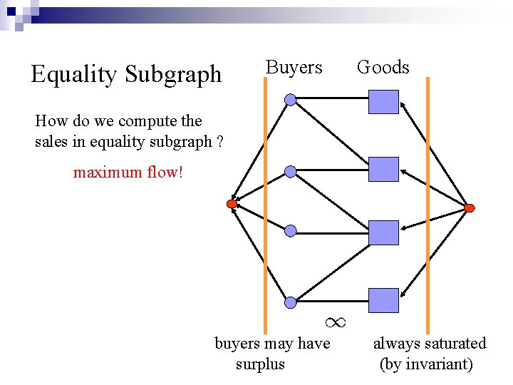
Equality Subgraph Buyers Goods How do we compute the sales in equality subgraph ? maximum flow! buyers may have surplus always saturated (by invariant)

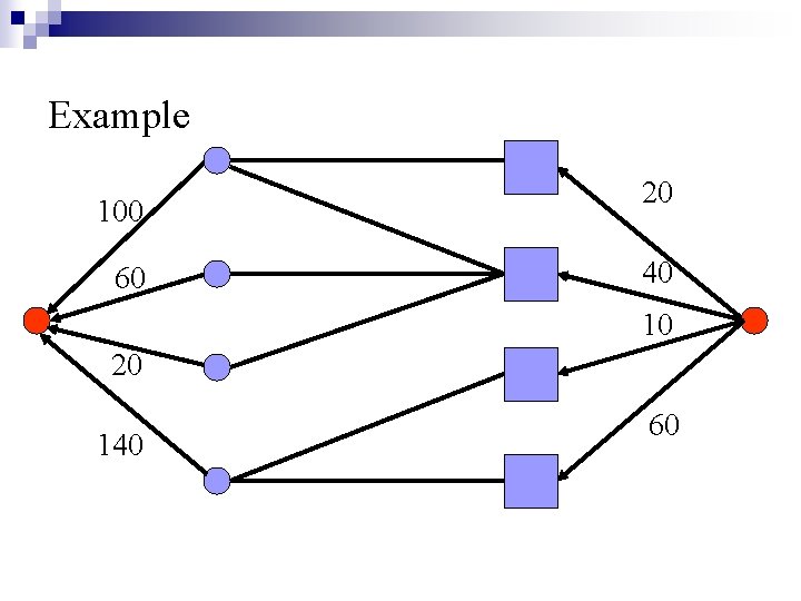
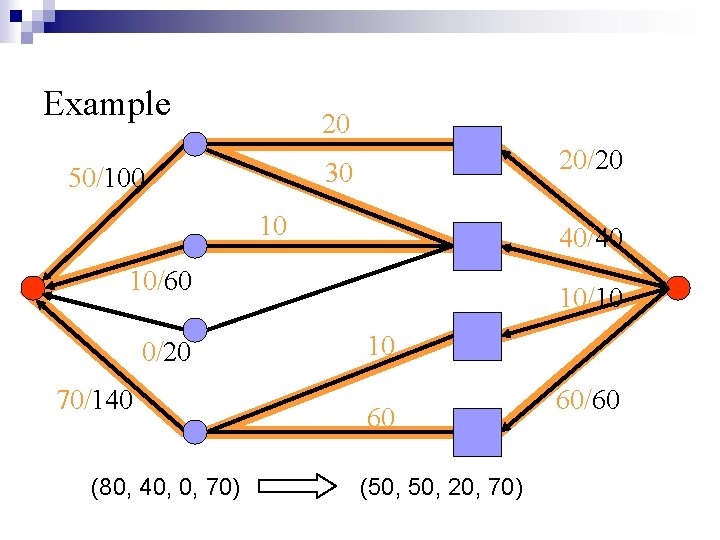
Example 100 60 20 40 10 20 140 60

Example 20 20/100 20 20/60 20/20 70/140 40/40 20 10/10 10 60 60/60

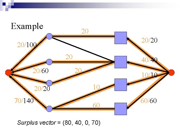
Example 20 20/100 20 20/60 20/20 70/140 40/40 20 10/10 10 60 Surplus vector = (80, 40, 0, 70) 60/60

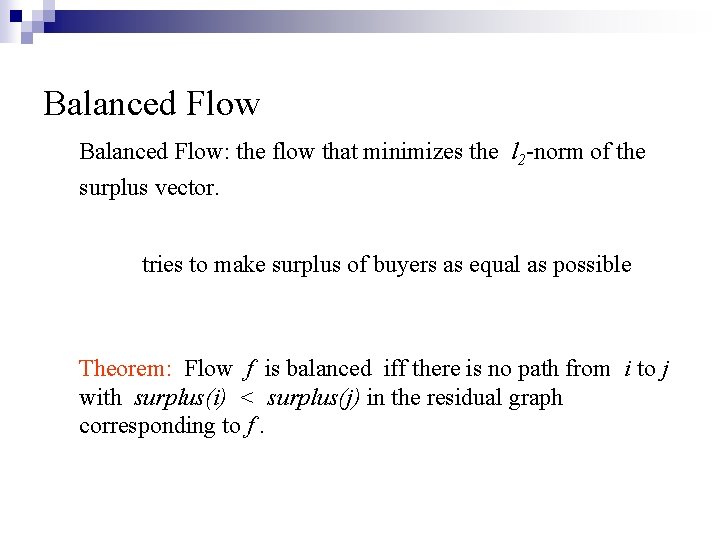
Balanced Flow: the flow that minimizes the l 2 -norm of the surplus vector. tries to make surplus of buyers as equal as possible Theorem: Flow f is balanced iff there is no path from i to j with surplus(i) < surplus(j) in the residual graph corresponding to f.

Example 20 20/100 20 20/60 20/20 70/140 40/40 20 10/10 10 60 Surplus vector = (80, 40, 0, 70) 60/60

Example 20 20/20 30 50/100 10 40/40 10/60 0/20 70/140 (80, 40, 0, 70) 10/10 10 60 (50, 20, 70) 60/60

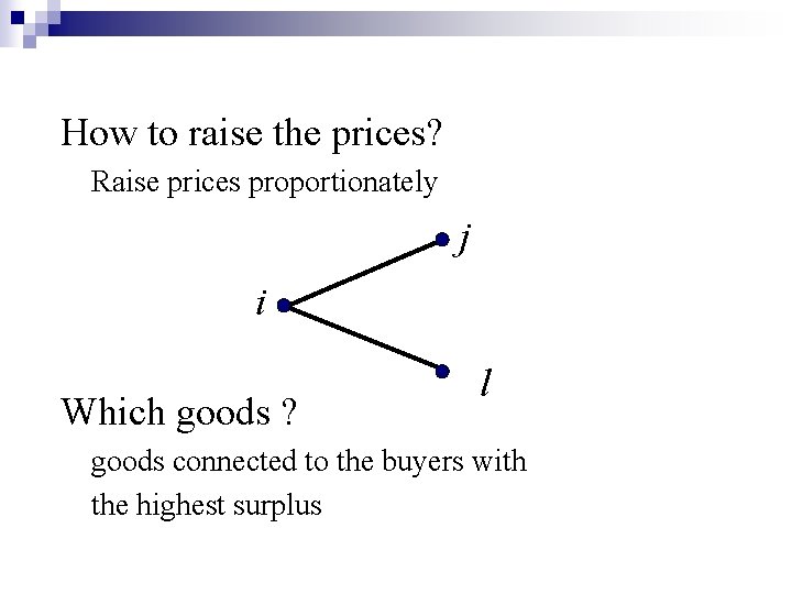
How to raise the prices? Raise prices proportionately j i Which goods ? l goods connected to the buyers with the highest surplus

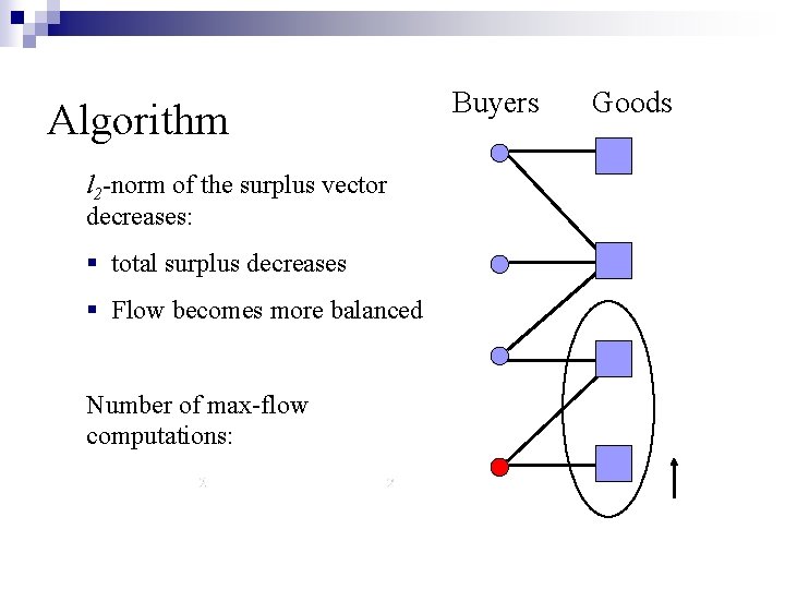
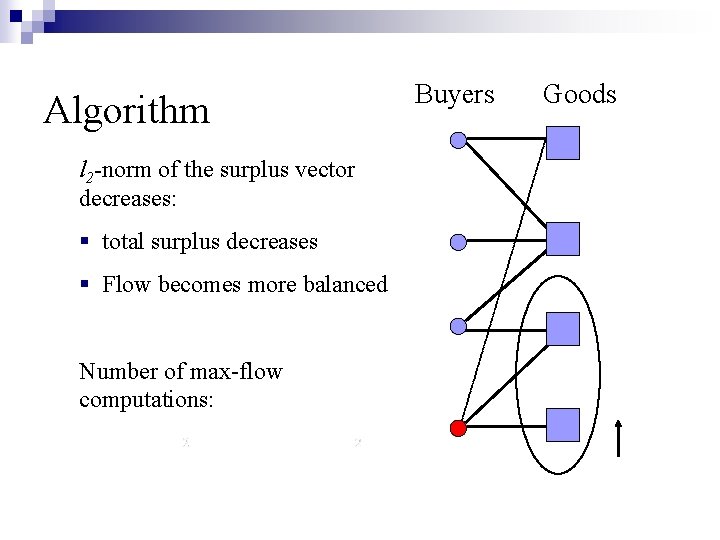
Algorithm l 2 -norm of the surplus vector decreases: § total surplus decreases § Flow becomes more balanced Number of max-flow computations: Buyers Goods

Algorithm l 2 -norm of the surplus vector decreases: § total surplus decreases § Flow becomes more balanced Number of max-flow computations: Buyers Goods

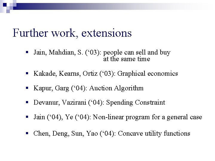
Further work, extensions § Jain, Mahdian, S. (‘ 03): people can sell and buy at the same time § Kakade, Kearns, Ortiz (‘ 03): Graphical economics § Kapur, Garg (‘ 04): Auction Algorithm § Devanur, Vazirani (‘ 04): Spending Constraint § Jain (‘ 04), Ye (‘ 04): Non-linear program for a general case § Chen, Deng, Sun, Yao (‘ 04): Concave utility functions

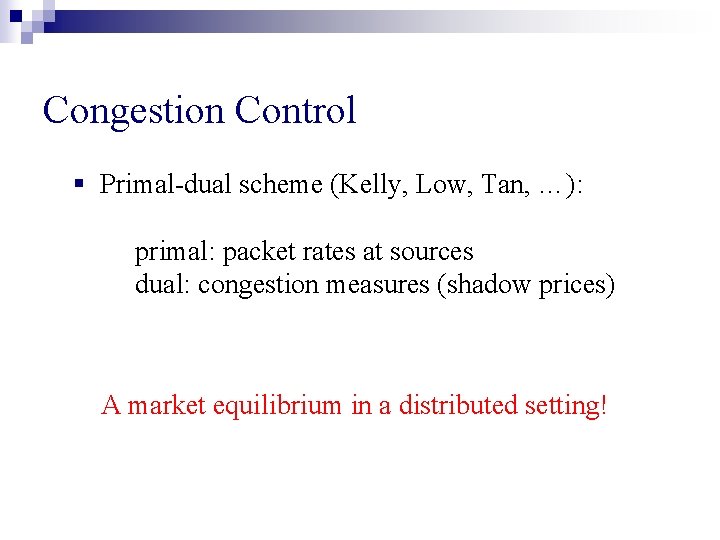
Congestion Control § Primal-dual scheme (Kelly, Low, Tan, …): primal: packet rates at sources dual: congestion measures (shadow prices) A market equilibrium in a distributed setting!

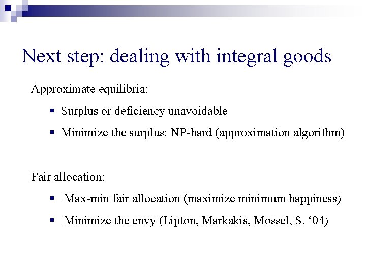
Next step: dealing with integral goods Approximate equilibria: § Surplus or deficiency unavoidable § Minimize the surplus: NP-hard (approximation algorithm) Fair allocation: § Max-min fair allocation (maximize minimum happiness) § Minimize the envy (Lipton, Markakis, Mossel, S. ‘ 04)

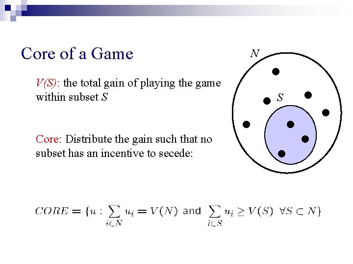
Core of a Game V(S): the total gain of playing the game within subset S Core: Distribute the gain such that no subset has an incentive to secede: N • S • •

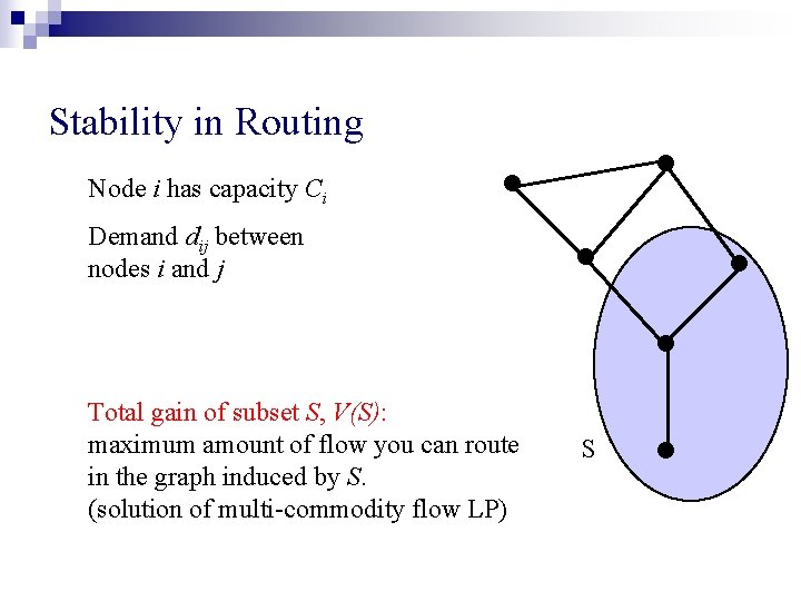
Stability in Routing Node i has capacity Ci • • Demand dij between nodes i and j • • • Total gain of subset S, V(S): maximum amount of flow you can route in the graph induced by S. (solution of multi-commodity flow LP) S •

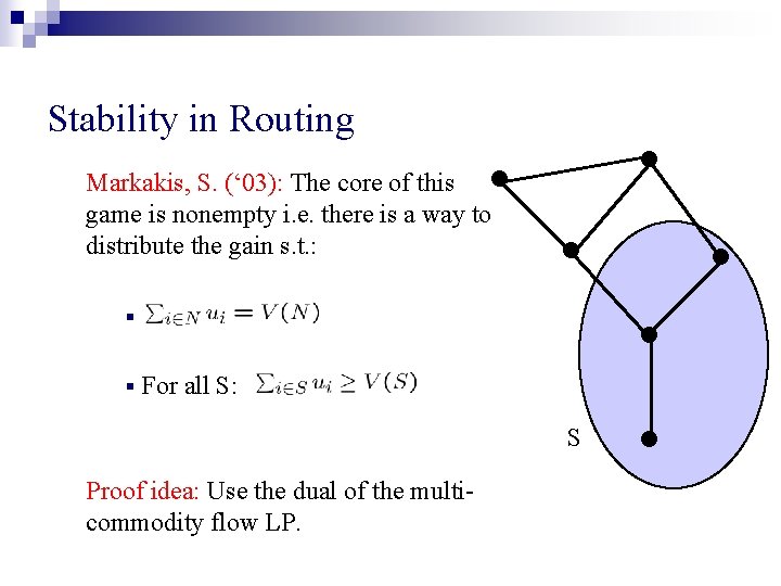
Stability in Routing • • Markakis, S. (‘ 03): The core of this game is nonempty i. e. there is a way to distribute the gain s. t. : • • § § • For all S: S Proof idea: Use the dual of the multicommodity flow LP. •

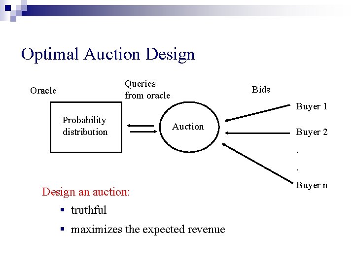
Optimal Auction Design Queries from oracle Oracle Probability distribution Bids Buyer 1 Auction Buyer 2. . Design an auction: § truthful § maximizes the expected revenue Buyer n

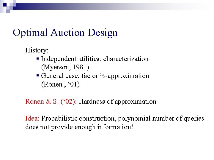
Optimal Auction Design History: § Independent utilities: characterization (Myerson, 1981) § General case: factor ½-approximation (Ronen , ‘ 01) Ronen & S. (‘ 02): Hardness of approximation Idea: Probabilistic construction; polynomial number of queries does not provide enough information!

Computer Science Applications: § networking: algorithms and protocols § E–commerce Game Theory Applications: § modeling, simulation § intrinsic complexity § bounded rationality

Outline n Game Theory and Algorithms efficient algorithms for game theoretic notions n Complex networks and performance of basic algorithms

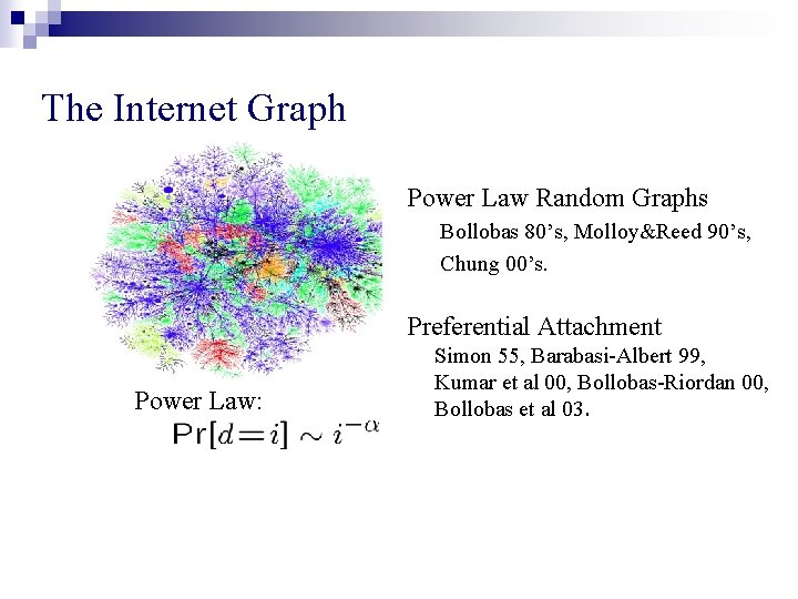
The Internet Graph Power Law Random Graphs Bollobas 80’s, Molloy&Reed 90’s, Chung 00’s. Preferential Attachment Power Law: Simon 55, Barabasi-Albert 99, Kumar et al 00, Bollobas-Riordan 00, Bollobas et al 03.

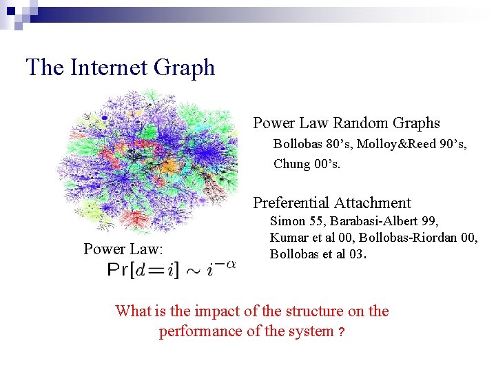
The Internet Graph Power Law Random Graphs Bollobas 80’s, Molloy&Reed 90’s, Chung 00’s. Preferential Attachment Power Law: Simon 55, Barabasi-Albert 99, Kumar et al 00, Bollobas-Riordan 00, Bollobas et al 03. What is the impact of the structure on the performance of the system ?

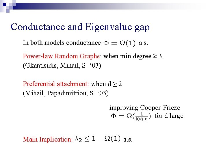
Conductance and Eigenvalue gap In both models conductance a. s. Power-law Random Graphs: when min degree ≥ 3. (Gkantisidis, Mihail, S. ‘ 03) Preferential attachment: when d ≥ 2 (Mihail, Papadimitriou, S. ‘ 03) improving Cooper-Frieze for d large Main Implication: a. s.

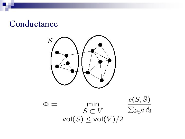
Conductance # Cut edges

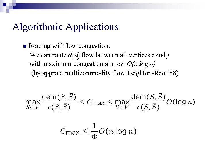
Algorithmic Applications n Routing with low congestion: We can route di dj flow between all vertices i and j with maximum congestion at most O(n log n). (by approx. multicommodity flow Leighton-Rao ‘ 88)

Algorithmic Applications n Bounds on mixing time, hitting time and cover time (searching and crawling) n Random walks for search and construction in P 2 P networks (Gkantsidis, Mihail, S. ‘ 04) n Search with replication in P 2 P networks generalizing the notion of cover time (Mihail, Tetali, S. , in preparation)

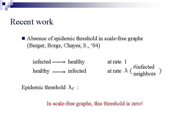
Recent work n Absence of epidemic threshold in scale-free graphs (Berger, Borgs, Chayes, S. , ‘ 04) infected healthy at rate 1 healthy infected at rate Epidemic threshold #infected ( neighbors ) : In scale-free graphs, this threshold is zero!

THE END !