CS 3343 Analysis of Algorithms Review for Exam

CS 3343: Analysis of Algorithms Review for Exam 2

Exam 2 • Closed book exam • One cheat sheet allowed (limit to a single page of letter-size paper, double-sided) • Tuesday, Nov 17, class time + 5 minutes • Basic calculator (no graphing) is allowed but not necessary

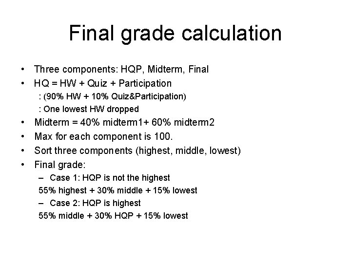
Final grade calculation • Three components: HQP, Midterm, Final • HQ = HW + Quiz + Participation : (90% HW + 10% Quiz&Participation) : One lowest HW dropped • • Midterm = 40% midterm 1+ 60% midterm 2 Max for each component is 100. Sort three components (highest, middle, lowest) Final grade: – Case 1: HQP is not the highest 55% highest + 30% middle + 15% lowest – Case 2: HQP is highest 55% middle + 30% HQP + 15% lowest

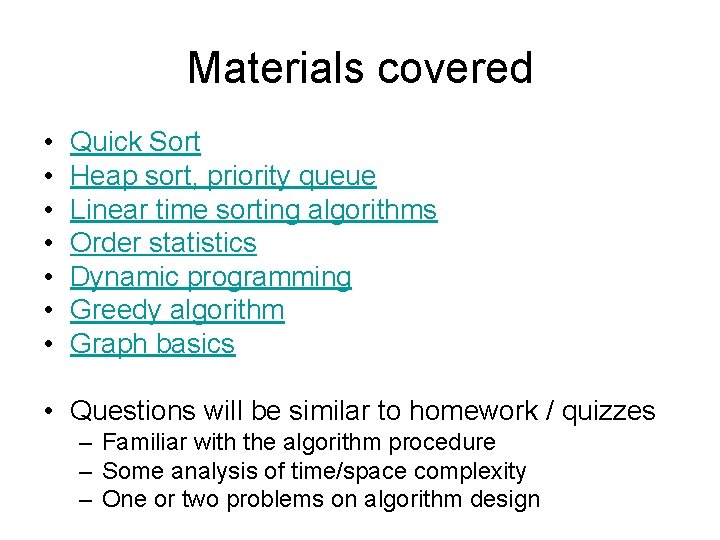
Materials covered • • Quick Sort Heap sort, priority queue Linear time sorting algorithms Order statistics Dynamic programming Greedy algorithm Graph basics • Questions will be similar to homework / quizzes – Familiar with the algorithm procedure – Some analysis of time/space complexity – One or two problems on algorithm design

Quick. Sort • • Quicksort algorithm Randimized Quicksort algorithm Partition algorithm Quicksort/Randomized Quicksort time complexity analysis Back

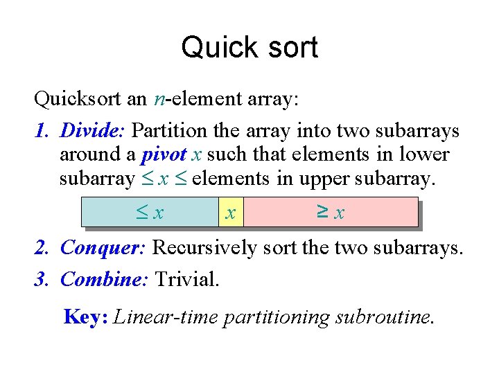
Quick sort Quicksort an n-element array: 1. Divide: Partition the array into two subarrays around a pivot x such that elements in lower subarray £ x £ elements in upper subarray. £x x ≥x 2. Conquer: Recursively sort the two subarrays. 3. Combine: Trivial. Key: Linear-time partitioning subroutine.

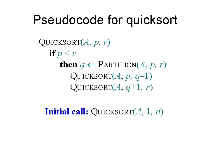
Pseudocode for quicksort QUICKSORT(A, p, r) if p < r then q PARTITION(A, p, r) QUICKSORT(A, p, q– 1) QUICKSORT(A, q+1, r) Initial call: QUICKSORT(A, 1, n)

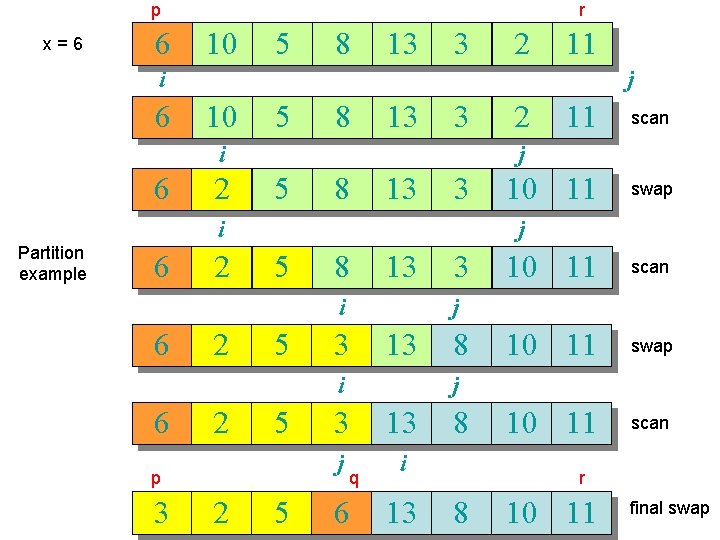
Partition Code Partition(A, p, r) x = A[p]; // pivot is the first element i = p; j = r + 1; while (TRUE) { repeat i++; until A[i] > x | i >= j; repeat j--; until A[j] < x | j <= i; if (i < j) Swap (A[i], A[j]); else break; } swap (A[p], A[j]); return j;

p x=6 6 r 10 5 8 13 3 2 11 i 6 j 10 5 8 13 3 i 6 2 5 8 13 3 2 5 5 p 3 2 10 11 swap 5 3 10 11 scan 10 11 swap 10 11 scan j 3 13 i 6 scan j i 6 11 j i Partition example 2 8 j 3 13 j i q 6 13 8 r 8 10 11 final swap

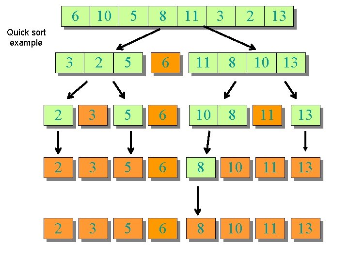
6 10 5 8 11 3 2 13 Quick sort example 3 2 5 6 11 8 10 13 2 3 5 6 10 8 11 13 2 3 5 6 8 10 11 13

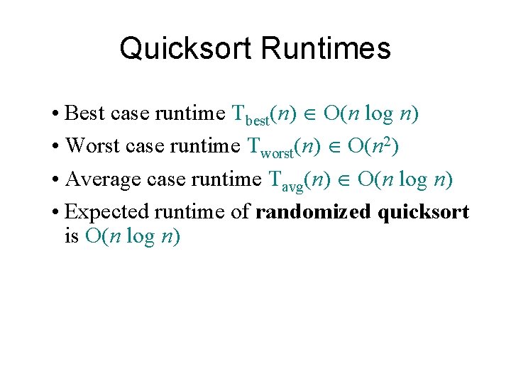
Quicksort Runtimes • Best case runtime Tbest(n) O(n log n) • Worst case runtime Tworst(n) O(n 2) • Average case runtime Tavg(n) O(n log n) • Expected runtime of randomized quicksort is O(n log n)

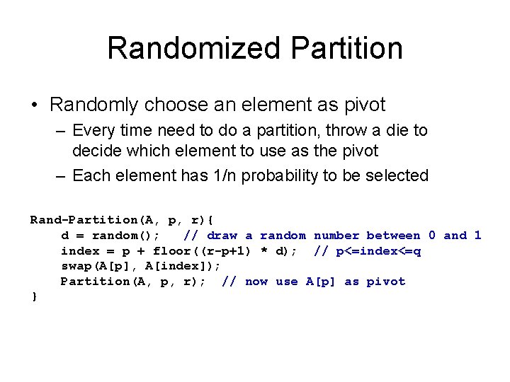
Randomized Partition • Randomly choose an element as pivot – Every time need to do a partition, throw a die to decide which element to use as the pivot – Each element has 1/n probability to be selected Rand-Partition(A, p, r){ d = random(); // draw a random number between 0 and 1 index = p + floor((r-p+1) * d); // p<=index<=q swap(A[p], A[index]); Partition(A, p, r); // now use A[p] as pivot }

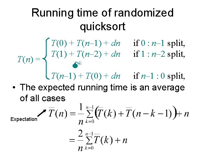
Running time of randomized quicksort T(0) + T(n– 1) + dn if 0 : n– 1 split, T(1) + T(n– 2) + dn if 1 : n– 2 split, T(n) = M T(n– 1) + T(0) + dn if n– 1 : 0 split, • The expected running time is an average of all cases Expectation

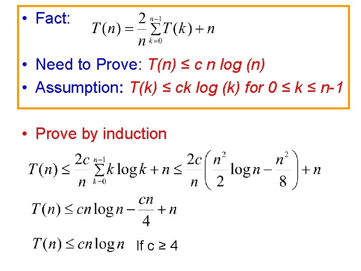
• Fact: • Need to Prove: T(n) ≤ c n log (n) • Assumption: T(k) ≤ ck log (k) for 0 ≤ k ≤ n-1 • Prove by induction If c ≥ 4

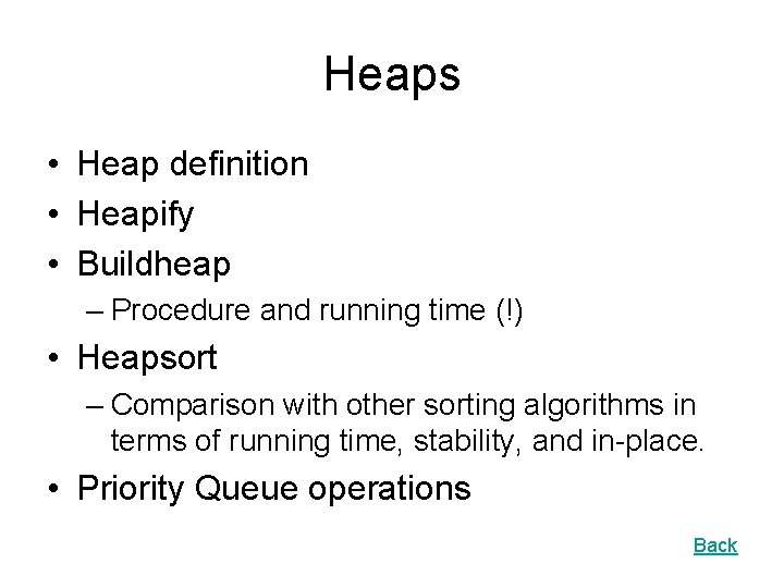
Heaps • Heap definition • Heapify • Buildheap – Procedure and running time (!) • Heapsort – Comparison with other sorting algorithms in terms of running time, stability, and in-place. • Priority Queue operations Back

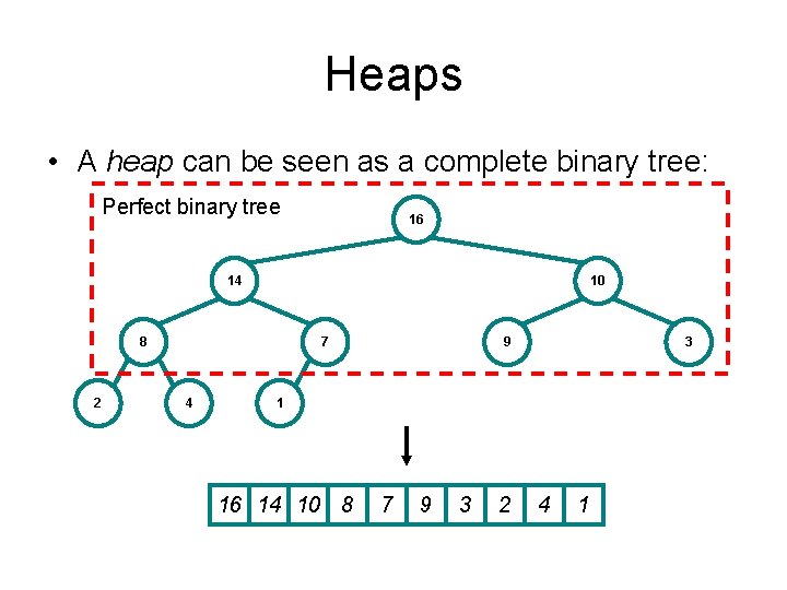
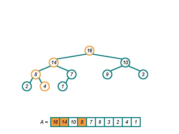
Heaps • A heap can be seen as a complete binary tree: Perfect binary tree 16 14 10 8 2 7 4 9 3 1 16 14 10 8 7 9 3 2 4 1

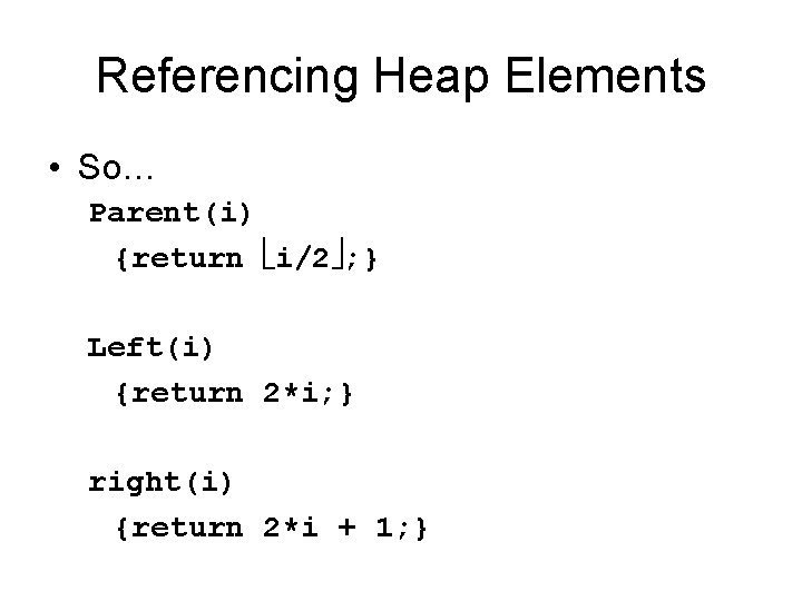
Referencing Heap Elements • So… Parent(i) {return i/2 ; } Left(i) {return 2*i; } right(i) {return 2*i + 1; }

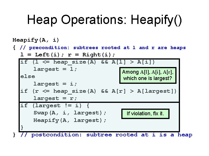
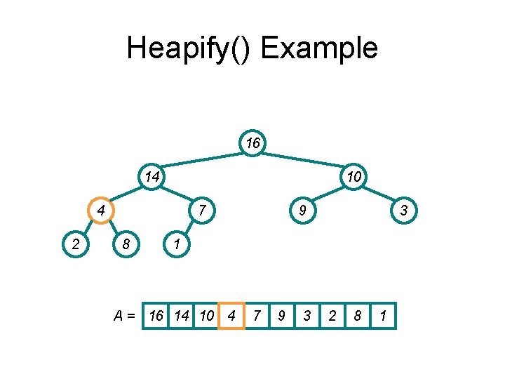
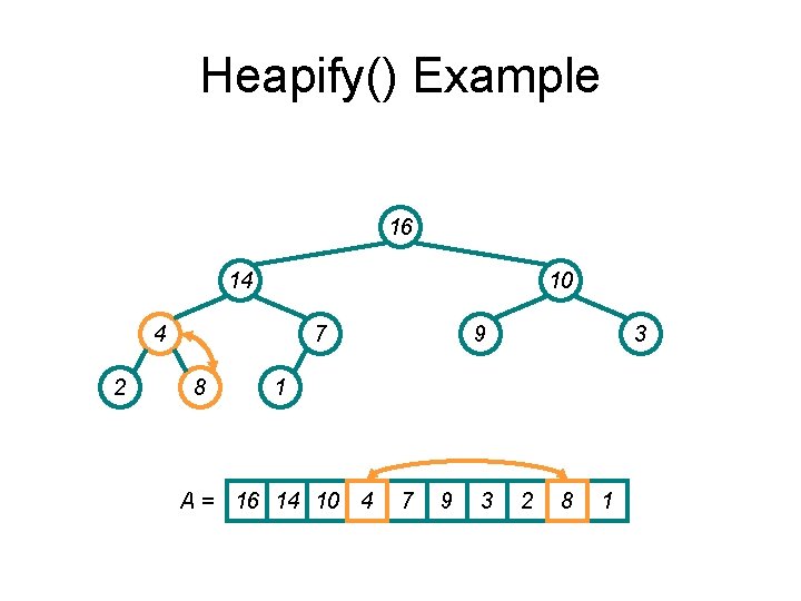
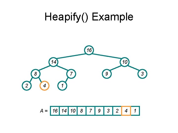
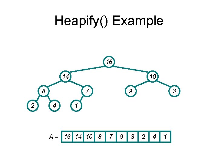
Heap Operations: Heapify() Heapify(A, i) { // precondition: subtrees rooted at l and r are heaps l = Left(i); r = Right(i); if (l <= heap_size(A) && A[l] > A[i]) largest = l; Among A[l], A[i], A[r], else which one is largest? largest = i; if (r <= heap_size(A) && A[r] > A[largest]) largest = r; if (largest != i) { Swap(A, i, largest); If violation, fix it. Heapify(A, largest); } } // postcondition: subtree rooted at i is a heap

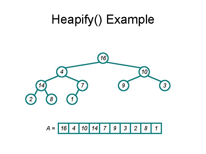
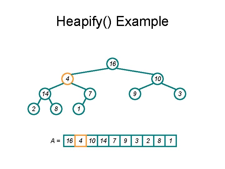
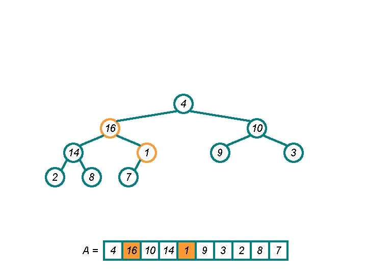
Heapify() Example 16 4 10 14 2 7 8 9 3 1 A = 16 4 10 14 7 9 3 2 8 1

Heapify() Example 16 4 10 14 2 7 8 9 3 1 A = 16 4 10 14 7 9 3 2 8 1

Heapify() Example 16 4 10 14 2 7 8 9 3 1 A = 16 4 10 14 7 9 3 2 8 1

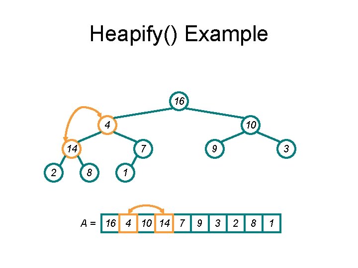
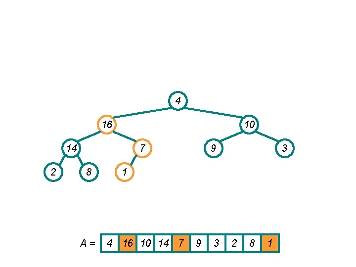
Heapify() Example 16 14 10 4 2 7 8 9 3 1 A = 16 14 10 4 7 9 3 2 8 1

Heapify() Example 16 14 10 4 2 7 8 9 3 1 A = 16 14 10 4 7 9 3 2 8 1

Heapify() Example 16 14 10 8 2 7 4 9 3 1 A = 16 14 10 8 7 9 3 2 4 1

Heapify() Example 16 14 10 8 2 7 4 9 3 1 A = 16 14 10 8 7 9 3 2 4 1

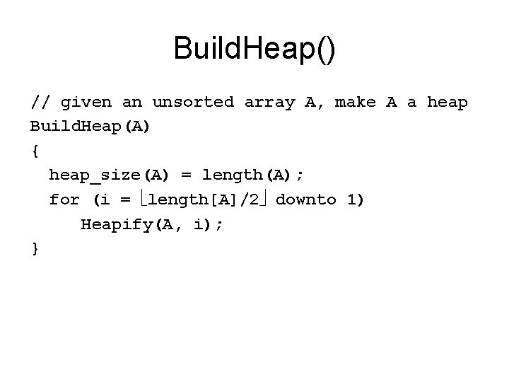
Build. Heap() // given an unsorted array A, make A a heap Build. Heap(A) { heap_size(A) = length(A); for (i = length[A]/2 downto 1) Heapify(A, i); }

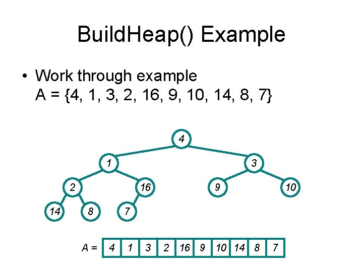
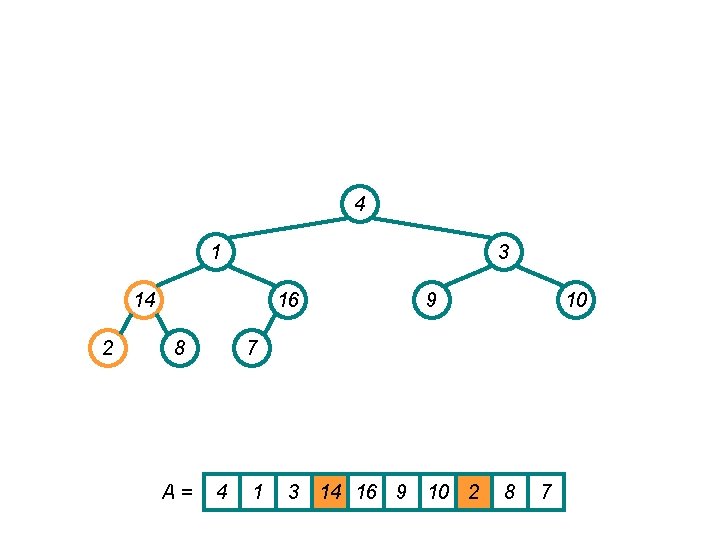
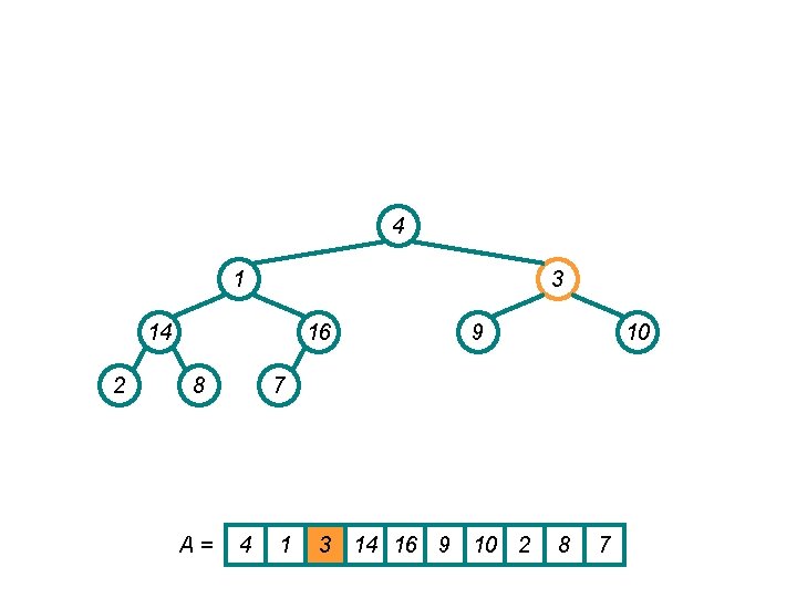
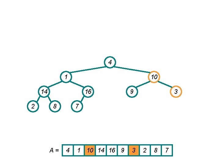
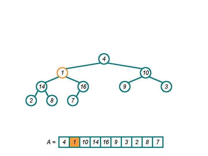
Build. Heap() Example • Work through example A = {4, 1, 3, 2, 16, 9, 10, 14, 8, 7} 4 1 3 2 14 16 8 A= 9 10 7 4 1 3 2 16 9 10 14 8 7

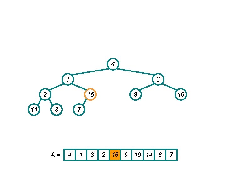
4 1 3 2 14 16 8 A= 9 10 7 4 1 3 2 16 9 10 14 8 7

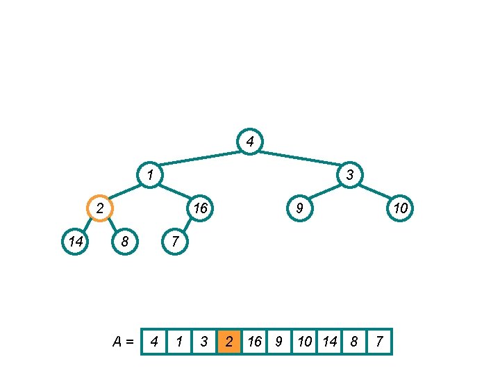
4 1 3 2 14 16 8 A= 9 10 7 4 1 3 2 16 9 10 14 8 7

4 1 3 14 2 16 8 A= 9 10 7 4 1 3 14 16 9 10 2 8 7

4 1 3 14 2 16 8 A= 9 10 7 4 1 3 14 16 9 10 2 8 7

4 1 10 14 2 16 8 A= 9 3 7 4 1 10 14 16 9 3 2 8 7

4 1 10 14 2 16 8 A= 9 3 7 4 1 10 14 16 9 3 2 8 7

4 16 10 14 2 1 8 A= 9 3 7 4 16 10 14 1 9 3 2 8 7

4 16 10 14 2 7 8 A= 9 3 1 4 16 10 14 7 9 3 2 8 1

4 16 10 14 2 7 8 A= 9 3 1 4 16 10 14 7 9 3 2 8 1

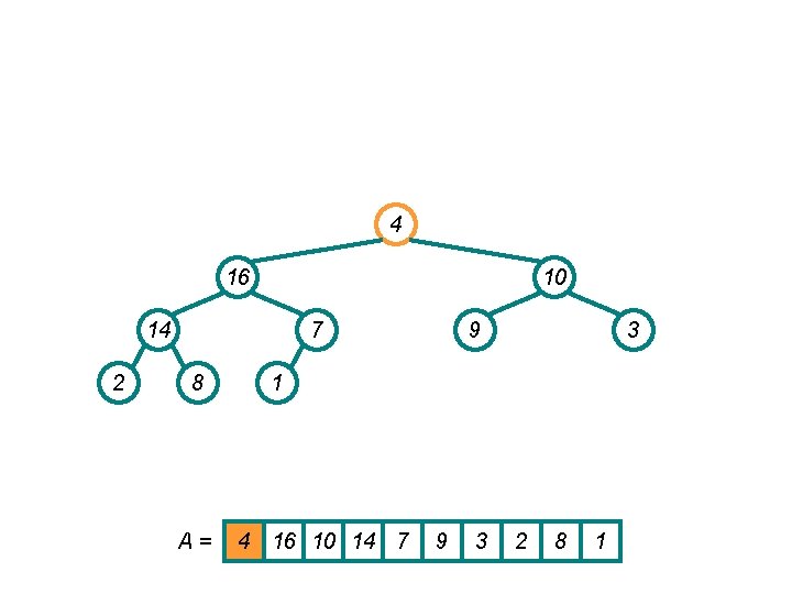
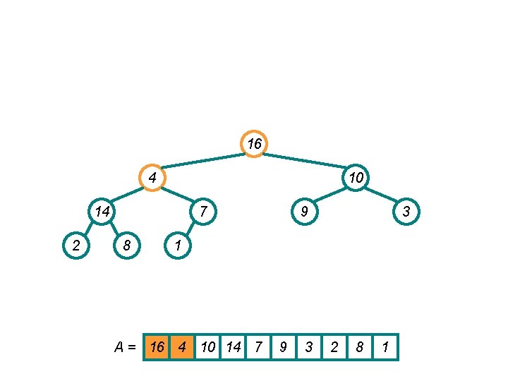
16 4 10 14 2 7 8 9 3 1 A = 16 4 10 14 7 9 3 2 8 1

16 14 10 4 2 7 8 9 3 1 A = 16 14 10 4 7 9 3 2 8 1

16 14 10 8 2 7 4 9 3 1 A = 16 14 10 8 7 9 3 2 4 1

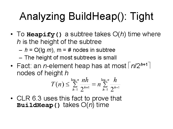
Analyzing Build. Heap(): Tight • To Heapify() a subtree takes O(h) time where h is the height of the subtree – h = O(lg m), m = # nodes in subtree – The height of most subtrees is small • Fact: an n-element heap has at most n/2 h+1 nodes of height h • CLR 6. 3 uses this fact to prove that Build. Heap() takes O(n) time

Heapsort(A) { Build. Heap(A); for (i = length(A) downto 2) { Swap(A[1], A[i]); heap_size(A) -= 1; Heapify(A, 1); } }

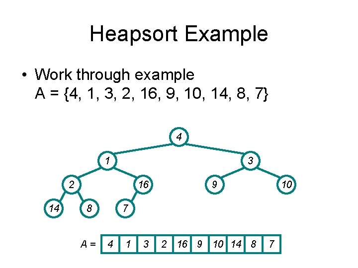
Heapsort Example • Work through example A = {4, 1, 3, 2, 16, 9, 10, 14, 8, 7} 4 1 3 2 14 16 8 A= 9 10 7 4 1 3 2 16 9 10 14 8 7

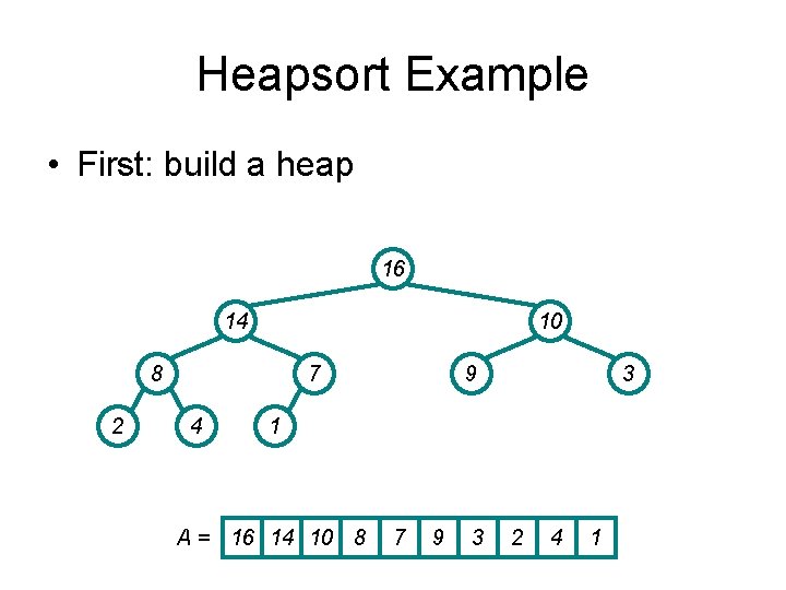
Heapsort Example • First: build a heap 16 14 10 8 2 7 4 9 3 1 A = 16 14 10 8 7 9 3 2 4 1

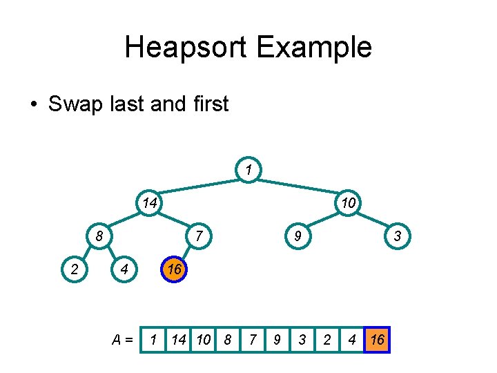
Heapsort Example • Swap last and first 1 14 10 8 2 7 4 A= 9 3 16 1 14 10 8 7 9 3 2 4 16

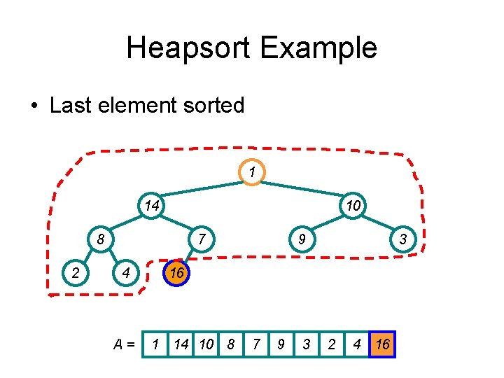
Heapsort Example • Last element sorted 1 14 10 8 2 7 4 A= 9 3 16 1 14 10 8 7 9 3 2 4 16

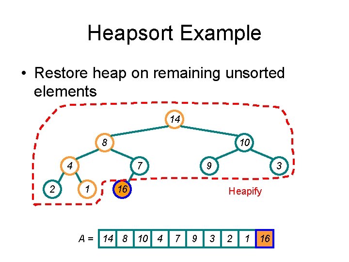
Heapsort Example • Restore heap on remaining unsorted elements 14 8 10 4 2 7 1 9 16 A = 14 8 10 4 3 Heapify 7 9 3 2 1 16

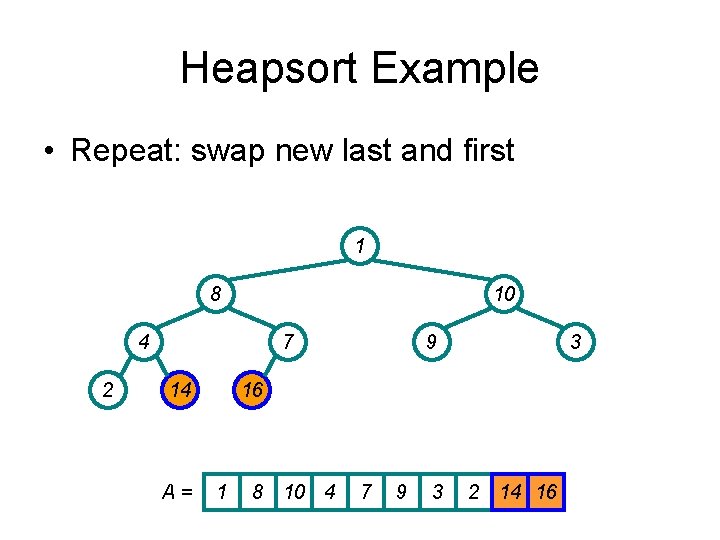
Heapsort Example • Repeat: swap new last and first 1 8 10 4 2 7 14 A= 9 3 16 1 8 10 4 7 9 3 2 14 16

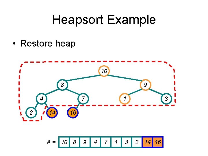
Heapsort Example • Restore heap 10 8 9 4 2 7 14 1 3 16 A = 10 8 9 4 7 1 3 2 14 16

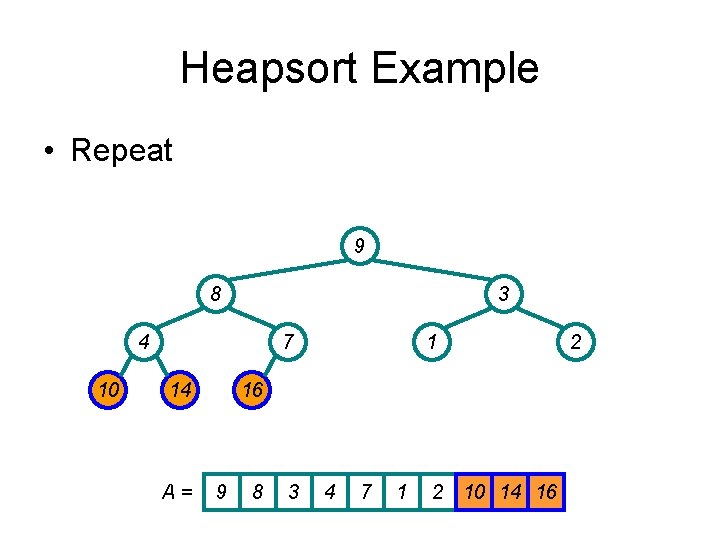
Heapsort Example • Repeat 9 8 3 4 10 7 14 A= 1 16 9 8 3 4 7 1 2 10 14 16 2

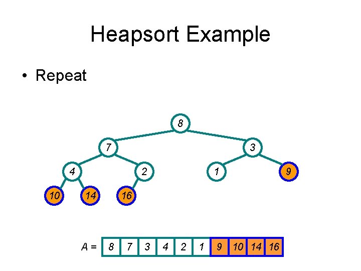
Heapsort Example • Repeat 8 7 3 4 10 2 14 A= 1 16 8 7 3 4 2 1 9 10 14 16 9

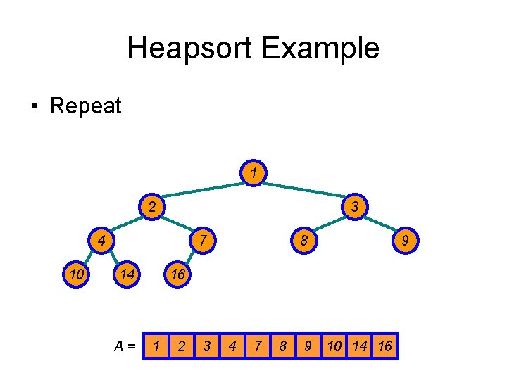
Heapsort Example • Repeat 1 2 3 4 10 7 14 A= 8 16 1 2 3 4 7 8 9 10 14 16 9

Implementing Priority Queues Heap. Maximum(A) { return A[1]; }

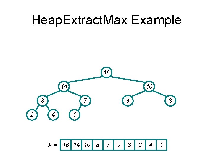
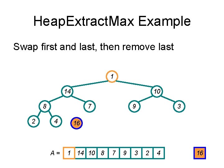
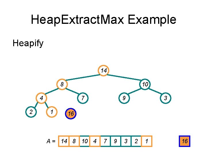
Implementing Priority Queues Heap. Extract. Max(A) { if (heap_size[A] < 1) { error; } max = A[1]; A[1] = A[heap_size[A]] heap_size[A] --; Heapify(A, 1); return max; }

Heap. Extract. Max Example 16 14 10 8 2 7 4 9 3 1 A = 16 14 10 8 7 9 3 2 4 1

Heap. Extract. Max Example Swap first and last, then remove last 1 14 10 8 2 7 4 A= 9 3 16 1 14 10 8 7 9 3 2 4 16

Heap. Extract. Max Example Heapify 14 8 10 4 2 7 1 9 3 16 A = 14 8 10 4 7 9 3 2 1 16

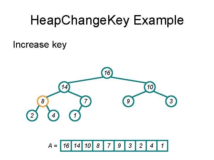
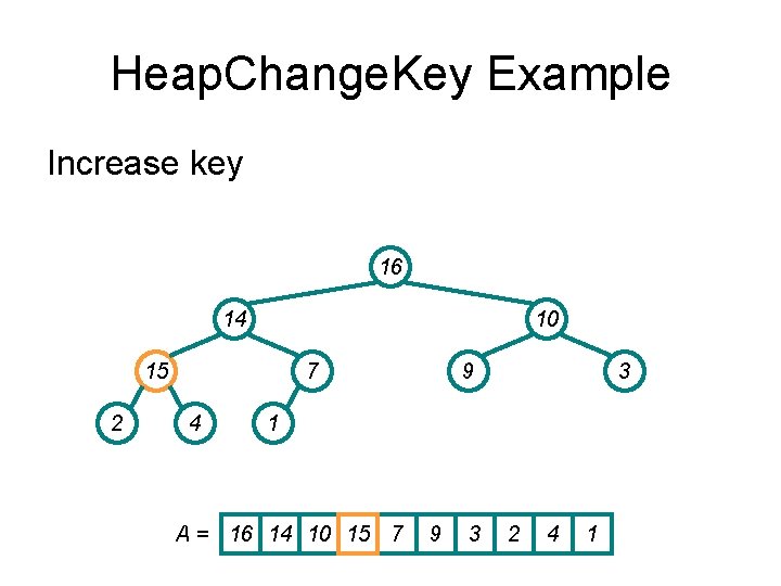
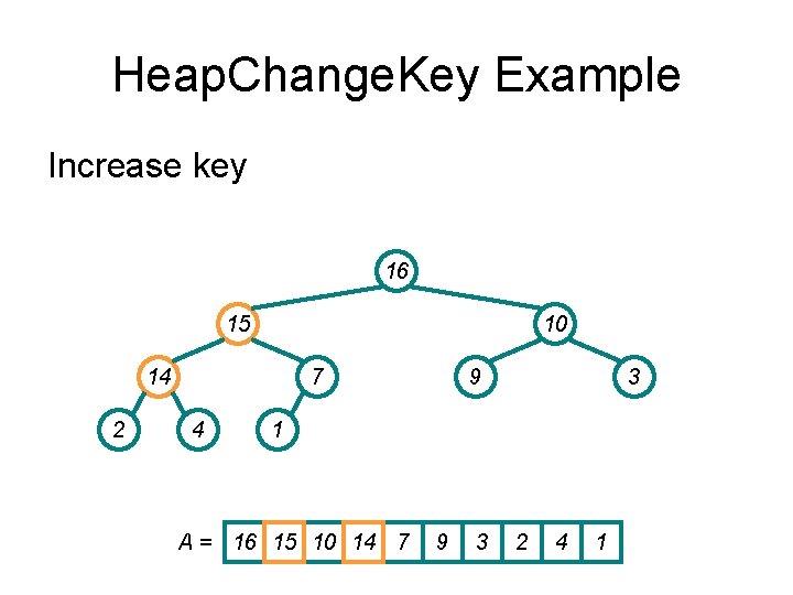
Implementing Priority Queues Heap. Change. Key(A, i, key){ if (key ≤ A[i]){ // decrease key A[i] = key; Sift down heapify(A, i); } else { // increase key A[i] = key; Bubble up while (i>1 & A[parent(i)]<A[i]) swap(A[i], A[parent(i)]; } }

Heap. Change. Key Example Increase key 16 14 10 8 2 7 4 9 3 1 A = 16 14 10 8 7 9 3 2 4 1

Heap. Change. Key Example Increase key 16 14 10 15 2 7 4 9 3 1 A = 16 14 10 15 7 9 3 2 4 1

Heap. Change. Key Example Increase key 16 15 10 14 2 7 4 9 3 1 A = 16 15 10 14 7 9 3 2 4 1

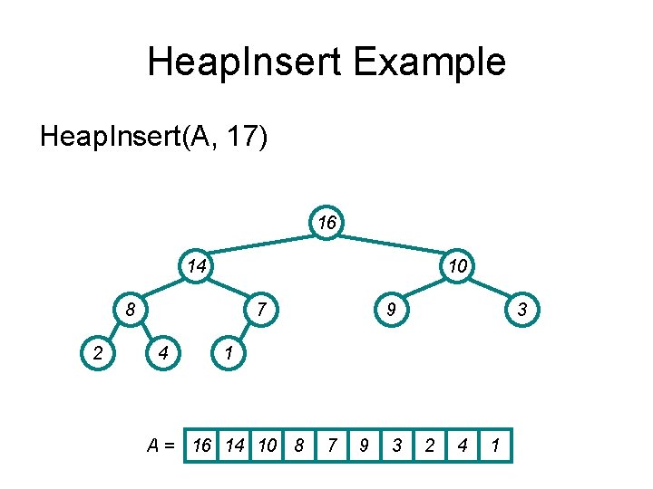
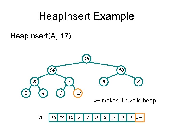
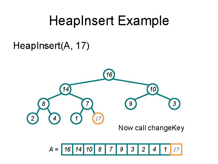
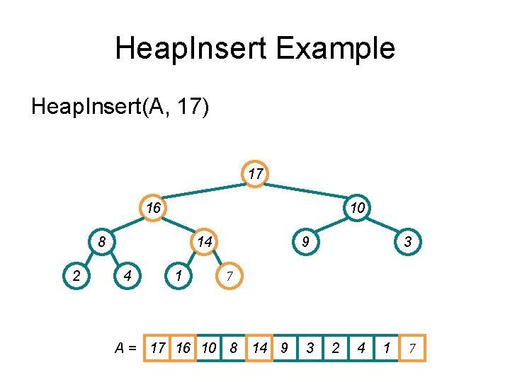
Implementing Priority Queues Heap. Insert(A, key) { heap_size[A] ++; i = heap_size[A]; A[i] = -∞; Heap. Change. Key(A, i, key); }

Heap. Insert Example Heap. Insert(A, 17) 16 14 10 8 2 7 4 9 3 1 A = 16 14 10 8 7 9 3 2 4 1

Heap. Insert Example Heap. Insert(A, 17) 16 14 10 8 2 7 4 1 9 3 -∞ -∞ makes it a valid heap A = 16 14 10 8 7 9 3 2 4 1 -∞

Heap. Insert Example Heap. Insert(A, 17) 16 14 10 8 2 7 4 1 9 3 17 Now call change. Key A = 16 14 10 8 7 9 3 2 4 1 17

Heap. Insert Example Heap. Insert(A, 17) 17 16 10 8 2 14 4 1 9 3 7 A = 17 16 10 8 14 9 3 2 4 1 7

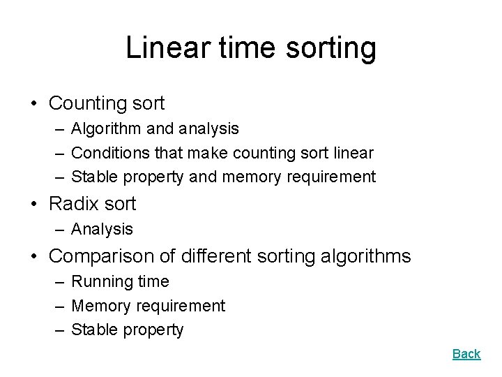
Linear time sorting • Counting sort – Algorithm and analysis – Conditions that make counting sort linear – Stable property and memory requirement • Radix sort – Analysis • Comparison of different sorting algorithms – Running time – Memory requirement – Stable property Back

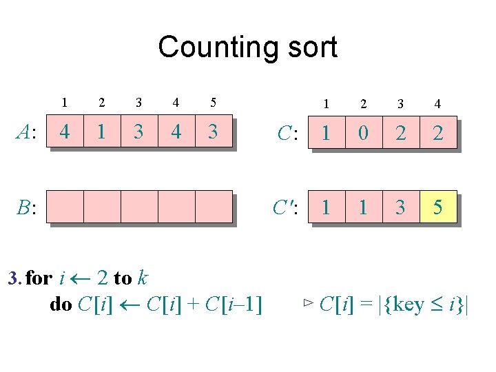
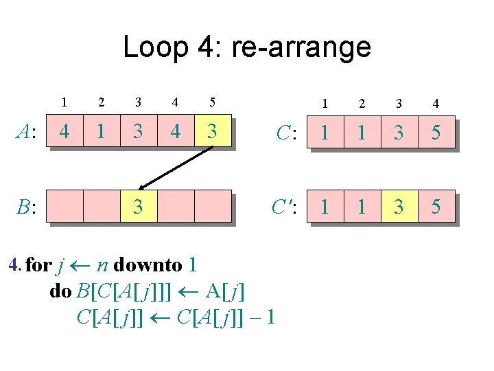
Counting sort 1. for i 1 to k Initialize do C[i] 0 Count 2. for j 1 to n do C[A[ j]] + 1 ⊳ C[i] = |{key = i}| Compute running sum 3. for i 2 to k do C[i] + C[i– 1] ⊳ C[i] = |{key £ i}| 4. for j n downto 1 Re-arrange do B[C[A[ j]]] A[ j] C[A[ j]] – 1

Counting sort A: 1 2 3 4 5 4 1 3 4 3 B: 3. for i 2 to k do C[i] + C[i– 1] 1 2 3 4 C: 1 0 2 2 C': 1 1 3 5 ⊳ C[i] = |{key £ i}|

Loop 4: re-arrange A: B: 1 2 3 4 5 4 1 3 4 3 3 4. for j n downto 1 1 2 3 4 C: 1 1 3 5 C': 1 1 3 5 do B[C[A[ j]]] A[ j] C[A[ j]] – 1

Analysis (k) (n) (n + k) 1. for i 1 to k do C[i] 0 2. for j 1 to n do C[A[ j]] + 1 3. for i 2 to k do C[i] + C[i– 1] 4. for j n downto 1 do B[C[A[ j]]] A[ j] C[A[ j]] – 1

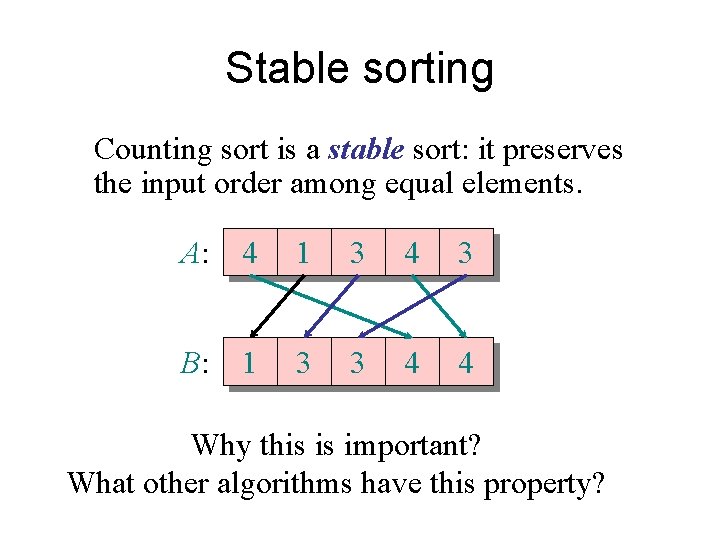
Stable sorting Counting sort is a stable sort: it preserves the input order among equal elements. A: 4 1 3 4 3 B: 1 3 3 4 4 Why this is important? What other algorithms have this property?

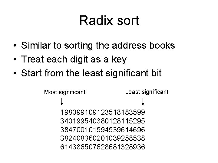
Radix sort • Similar to sorting the address books • Treat each digit as a key • Start from the least significant bit Most significant Least significant 198099109123518183599 340199540380128115295 384700101594539614696 382408360201039258538 614386507628681328936

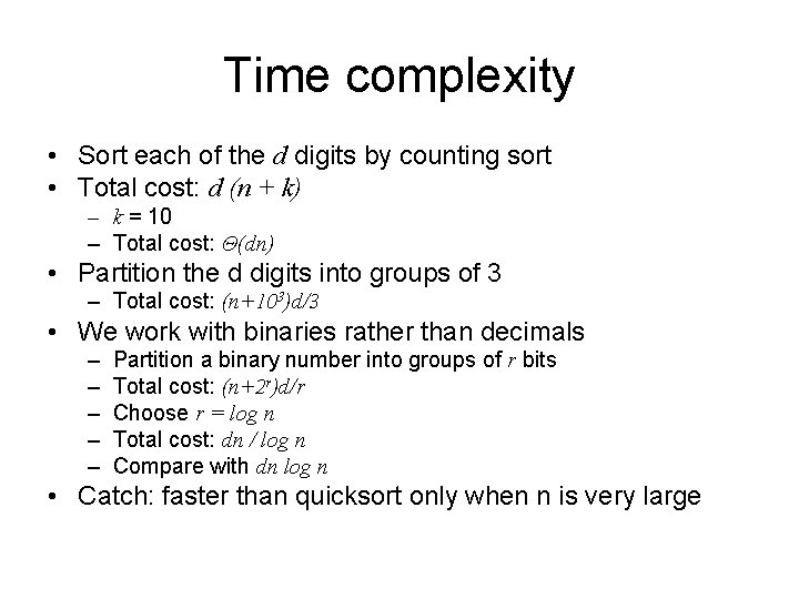
Time complexity • Sort each of the d digits by counting sort • Total cost: d (n + k) – k = 10 – Total cost: Θ(dn) • Partition the d digits into groups of 3 – Total cost: (n+103)d/3 • We work with binaries rather than decimals – – – Partition a binary number into groups of r bits Total cost: (n+2 r)d/r Choose r = log n Total cost: dn / log n Compare with dn log n • Catch: faster than quicksort only when n is very large

Order statistics • Select vs Randomize Select – Note: select is different from selection sort – Algorithm – Worst-case vs average-case (expected) running time analysis • Worst-case Linear-time Select – Algorithm and analysis – Comparison between sorting and select algorithms Back

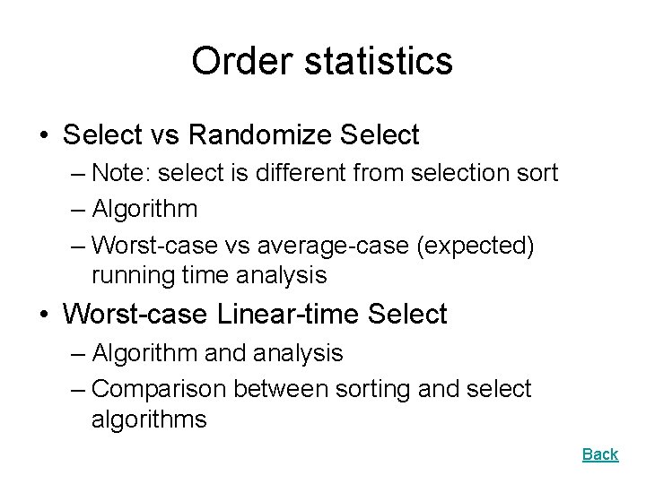
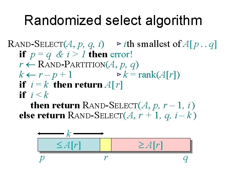
Randomized select algorithm RAND-SELECT(A, p, q, i) ⊳ i th smallest of A[ p. . q] if p = q & i > 1 then error! r RAND-PARTITION(A, p, q) k r–p+1 ⊳ k = rank(A[r]) if i = k then return A[ r] if i < k then return RAND-SELECT( A, p, r – 1, i ) else return RAND-SELECT( A, r + 1, q, i – k ) k £ A[r] p ³ A[r] r q

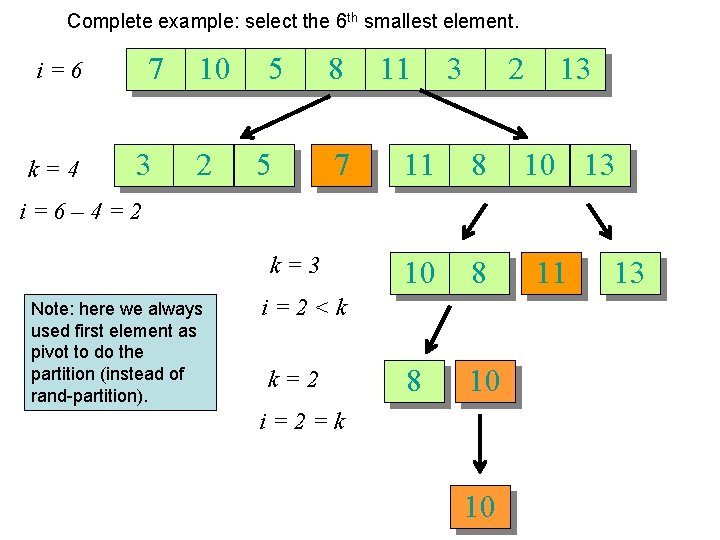
Complete example: select the 6 th smallest element. 7 i=6 k=4 3 10 2 5 5 8 7 11 3 2 11 8 10 8 8 10 13 i=6– 4=2 k=3 Note: here we always used first element as pivot to do the partition (instead of rand-partition). i=2<k k=2 i=2=k 10 11 13

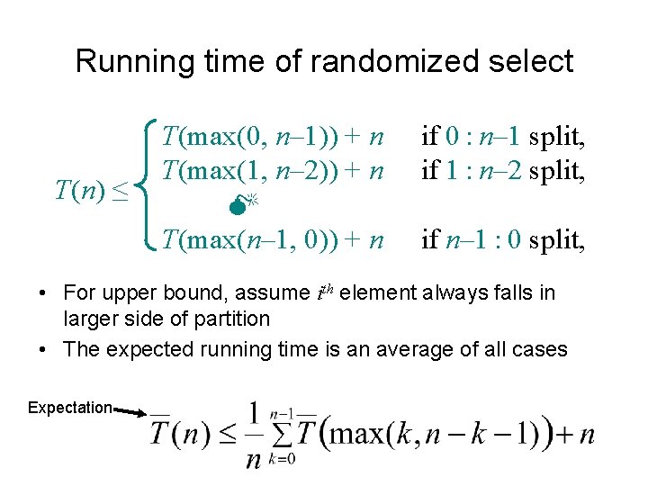
Running time of randomized select T(n) ≤ T(max(0, n– 1)) + n T(max(1, n– 2)) + n M T(max(n– 1, 0)) + n if 0 : n– 1 split, if 1 : n– 2 split, if n– 1 : 0 split, • For upper bound, assume ith element always falls in larger side of partition • The expected running time is an average of all cases Expectation

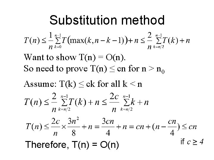
Substitution method Want to show T(n) = O(n). So need to prove T(n) ≤ cn for n > n 0 Assume: T(k) ≤ ck for all k < n Therefore, T(n) = O(n) if c ≥ 4

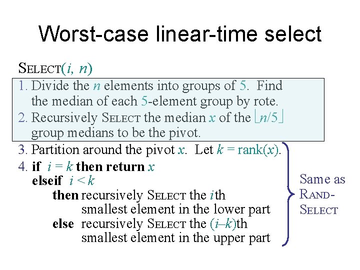
Worst-case linear-time select SELECT(i, n) 1. Divide the n elements into groups of 5. Find the median of each 5 -element group by rote. 2. Recursively SELECT the median x of the n/5 group medians to be the pivot. 3. Partition around the pivot x. Let k = rank(x). 4. if i = k then return x elseif i < k then recursively SELECT the i th smallest element in the lower part else recursively SELECT the (i–k)th smallest element in the upper part Same as RANDSELECT

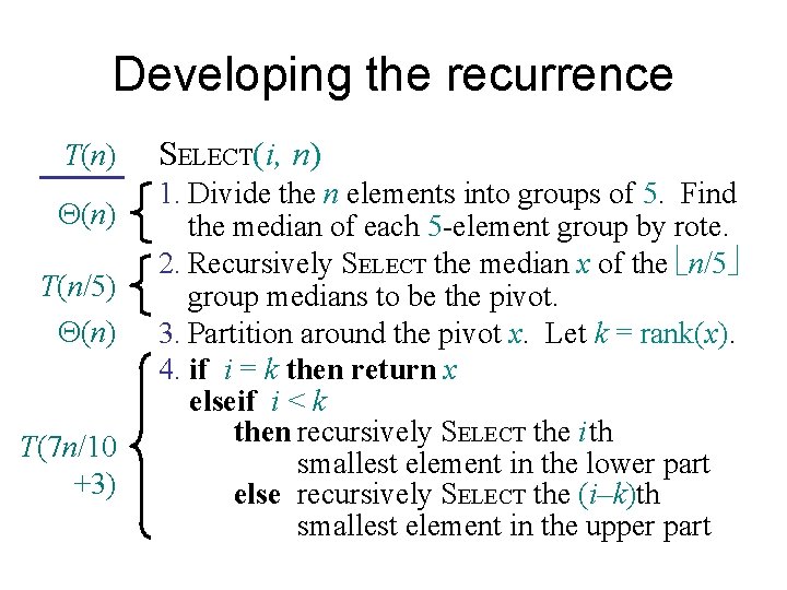
Developing the recurrence T(n) T(n/5) (n) T(7 n/10 +3) SELECT(i, n) 1. Divide the n elements into groups of 5. Find the median of each 5 -element group by rote. 2. Recursively SELECT the median x of the n/5 group medians to be the pivot. 3. Partition around the pivot x. Let k = rank(x). 4. if i = k then return x elseif i < k then recursively SELECT the i th smallest element in the lower part else recursively SELECT the (i–k)th smallest element in the upper part

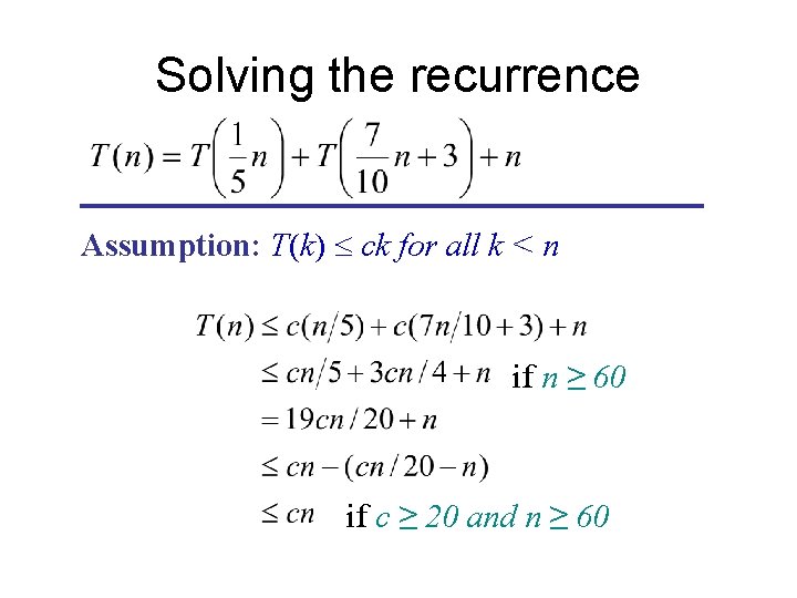
Solving the recurrence Assumption: T(k) £ ck for all k < n if n ≥ 60 if c ≥ 20 and n ≥ 60

Dynamic programming • • Proofs of optimal substructure property Defining recurrence Solve DP problem without recursive calls Example DP problems: – – – Shortest path problem LCS Restaurant location Knapsack Scheduling Other similar problems Back

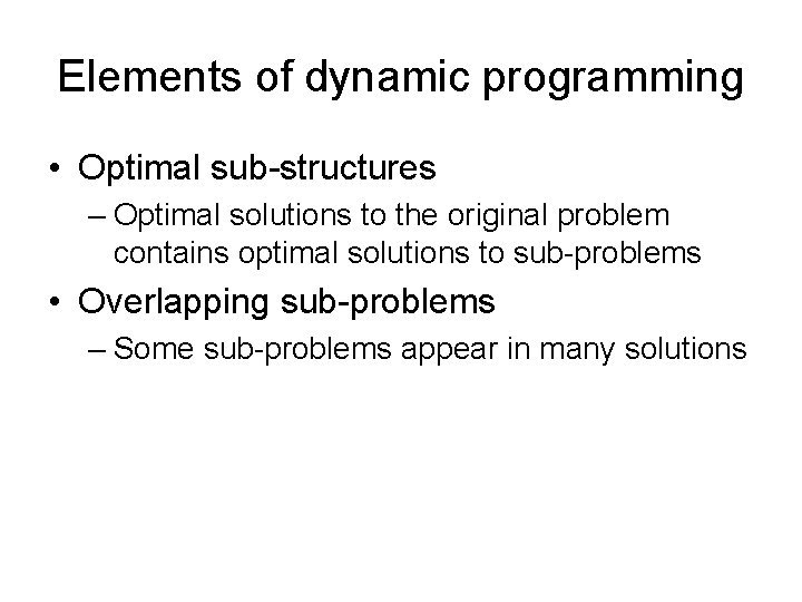
Elements of dynamic programming • Optimal sub-structures – Optimal solutions to the original problem contains optimal solutions to sub-problems • Overlapping sub-problems – Some sub-problems appear in many solutions

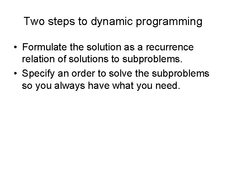
Two steps to dynamic programming • Formulate the solution as a recurrence relation of solutions to subproblems. • Specify an order to solve the subproblems so you always have what you need.

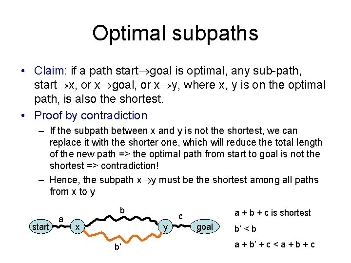
Optimal subpaths • Claim: if a path start goal is optimal, any sub-path, start x, or x goal, or x y, where x, y is on the optimal path, is also the shortest. • Proof by contradiction – If the subpath between x and y is not the shortest, we can replace it with the shorter one, which will reduce the total length of the new path => the optimal path from start to goal is not the shortest => contradiction! – Hence, the subpath x y must be the shortest among all paths from x to y start a b x y b’ a + b + c is shortest c goal b’ < b a + b’ + c < a + b + c

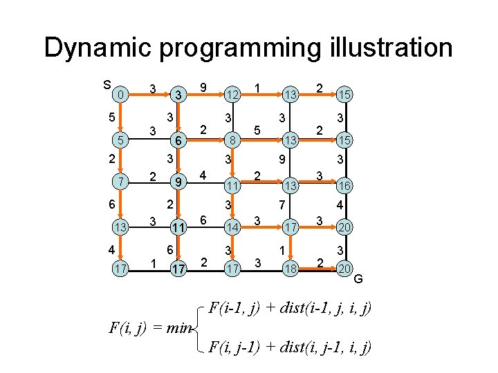
Dynamic programming illustration S 0 5 5 3 3 2 3 3 6 9 2 3 7 2 6 13 4 17 1 3 8 1 5 3 9 4 2 3 12 11 6 17 11 2 14 3 17 3 13 2 2 9 2 3 6 13 13 3 17 1 18 3 15 3 3 7 3 15 16 4 3 2 20 3 20 G F(i-1, j) + dist(i-1, j, i, j) F(i, j) = min F(i, j-1) + dist(i, j-1, i, j)

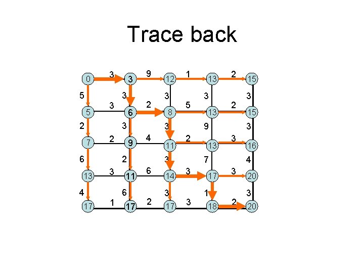
Trace back 0 5 5 3 3 2 3 3 6 9 2 3 7 2 6 13 4 17 1 3 8 1 5 3 9 4 2 3 12 11 6 17 11 2 14 3 17 3 13 2 2 9 2 3 6 13 13 3 17 1 18 3 15 3 3 7 3 15 16 4 3 2 20 3 20

Longest Common Subsequence • Given two sequences x[1. . m] and y[1. . n], find a longest subsequence common to them both. “a” not “the” x: A B C B D A y: B D C A B BCBA = LCS(x, y) functional notation, but not a function

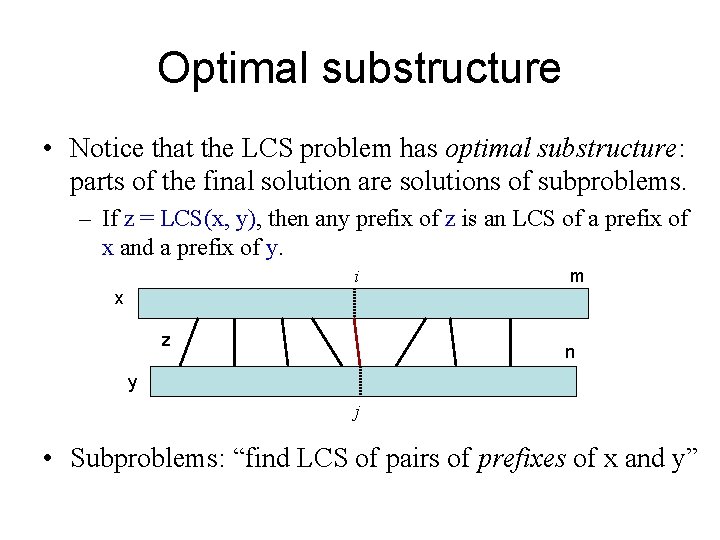
Optimal substructure • Notice that the LCS problem has optimal substructure: parts of the final solution are solutions of subproblems. – If z = LCS(x, y), then any prefix of z is an LCS of a prefix of x and a prefix of y. i m x z n y j • Subproblems: “find LCS of pairs of prefixes of x and y”

Finding length of LCS m x n y • Let c[i, j] be the length of LCS(x[1. . i], y[1. . j]) => c[m, n] is the length of LCS(x, y) • If x[m] = y[n] c[m, n] = c[m-1, n-1] + 1 • If x[m] != y[n] c[m, n] = max { c[m-1, n], c[m, n-1] }

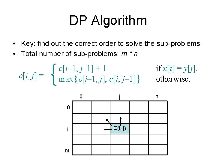
DP Algorithm • Key: find out the correct order to solve the sub-problems • Total number of sub-problems: m * n c[i, j] = c[i– 1, j– 1] + 1 max{c[i– 1, j], c[i, j– 1]} 0 j 0 i m C(i, j) if x[i] = y[j], otherwise. n

LCS Example (0) j i 0 X[i] 1 A 2 B 3 C 4 B 0 Y[j] 1 B 2 D X = ABCB; m = |X| = 4 Y = BDCAB; n = |Y| = 5 Allocate array c[5, 6] 3 C 4 A ABCB BDCAB 5 B

LCS Example (1) j i ABCB BDCAB 5 0 Y[j] 1 B 2 D 3 C 4 A B 0 0 0 X[i] 0 1 A 0 2 B 0 3 C 0 4 B 0 for i = 1 to m for j = 1 to n c[i, 0] = 0 c[0, j] = 0

LCS Example (2) j i ABCB BDCAB 5 0 Y[j] 1 B 2 D 3 C 4 A B 0 0 0 X[i] 0 0 1 A 0 0 2 B 0 3 C 0 4 B 0 if ( Xi == Yj ) c[i, j] = c[i-1, j-1] + 1 else c[i, j] = max( c[i-1, j], c[i, j-1] )

LCS Example (3) j i ABCB BDCAB 5 0 Y[j] 1 B 2 D 3 C 4 A B 0 0 0 X[i] 0 0 1 A 0 0 2 B 0 3 C 0 4 B 0 if ( Xi == Yj ) c[i, j] = c[i-1, j-1] + 1 else c[i, j] = max( c[i-1, j], c[i, j-1] )

LCS Example (4) j i ABCB BDCAB 5 0 Y[j] 1 B 2 D 3 C 4 A B 0 0 X[i] 0 0 0 1 A 0 0 1 2 B 0 3 C 0 4 B 0 if ( Xi == Yj ) c[i, j] = c[i-1, j-1] + 1 else c[i, j] = max( c[i-1, j], c[i, j-1] )

LCS Example (5) j i ABCB BDCAB 5 0 Y[j] 1 B 2 D 3 C 4 A B 0 X[i] 0 0 0 1 A 0 0 1 1 2 B 0 3 C 0 4 B 0 if ( Xi == Yj ) c[i, j] = c[i-1, j-1] + 1 else c[i, j] = max( c[i-1, j], c[i, j-1] )

LCS Example (6) j i ABCB BDCAB 5 0 Y[j] 1 B 2 D 3 C 4 A B 0 X[i] 0 0 0 1 A 0 0 1 1 2 B 0 1 3 C 0 4 B 0 if ( Xi == Yj ) c[i, j] = c[i-1, j-1] + 1 else c[i, j] = max( c[i-1, j], c[i, j-1] )

LCS Example (7) j i ABCB BDCAB 5 0 Y[j] 1 B 2 D 3 C 4 A B 0 X[i] 0 0 0 1 A 0 0 1 1 2 B 0 1 1 3 C 0 4 B 0 if ( Xi == Yj ) c[i, j] = c[i-1, j-1] + 1 else c[i, j] = max( c[i-1, j], c[i, j-1] )

LCS Example (8) j i ABCB BDCAB 5 0 Y[j] 1 B 2 D 3 C 4 A B 0 X[i] 0 0 0 1 A 0 0 1 1 2 B 0 1 1 2 3 C 0 4 B 0 if ( Xi == Yj ) c[i, j] = c[i-1, j-1] + 1 else c[i, j] = max( c[i-1, j], c[i, j-1] )

LCS Example (9) j i ABCB BDCAB 5 0 Y[j] 1 B 2 D 3 C 4 A B 0 X[i] 0 0 0 1 A 0 0 1 1 2 B 0 1 1 2 3 C 0 1 1 4 B 0 if ( Xi == Yj ) c[i, j] = c[i-1, j-1] + 1 else c[i, j] = max( c[i-1, j], c[i, j-1] )

LCS Example (10) j i ABCB BDCAB 5 0 Y[j] 1 B 2 D 3 C 4 A B 0 X[i] 0 0 0 1 A 0 0 1 1 2 B 0 1 1 2 3 C 0 1 1 2 4 B 0 if ( Xi == Yj ) c[i, j] = c[i-1, j-1] + 1 else c[i, j] = max( c[i-1, j], c[i, j-1] )

LCS Example (11) j i ABCB BDCAB 5 0 Y[j] 1 B 2 D 3 C 4 A B 0 X[i] 0 0 0 1 A 0 0 1 1 2 B 0 1 1 2 3 C 0 1 1 2 2 2 4 B 0 if ( Xi == Yj ) c[i, j] = c[i-1, j-1] + 1 else c[i, j] = max( c[i-1, j], c[i, j-1] )

LCS Example (12) j i ABCB BDCAB 5 0 Y[j] 1 B 2 D 3 C 4 A B 0 X[i] 0 0 0 1 A 0 0 1 1 2 B 0 1 1 2 3 C 0 1 1 2 2 2 4 B 0 1 if ( Xi == Yj ) c[i, j] = c[i-1, j-1] + 1 else c[i, j] = max( c[i-1, j], c[i, j-1] )

LCS Example (13) j i ABCB BDCAB 5 0 Y[j] 1 B 2 D 3 C 4 A B 0 X[i] 0 0 0 1 A 0 0 1 1 2 B 0 1 1 2 3 C 0 1 1 2 2 2 4 B 0 1 1 2 2 if ( Xi == Yj ) c[i, j] = c[i-1, j-1] + 1 else c[i, j] = max( c[i-1, j], c[i, j-1] )

LCS Example (14) j i ABCB BDCAB 5 0 Y[j] 1 B 2 D 3 C 4 A B 0 X[i] 0 0 0 1 A 0 0 1 1 2 B 0 1 1 2 3 C 0 1 1 2 2 2 4 B 0 1 1 2 2 3 if ( Xi == Yj ) c[i, j] = c[i-1, j-1] + 1 else c[i, j] = max( c[i-1, j], c[i, j-1] )

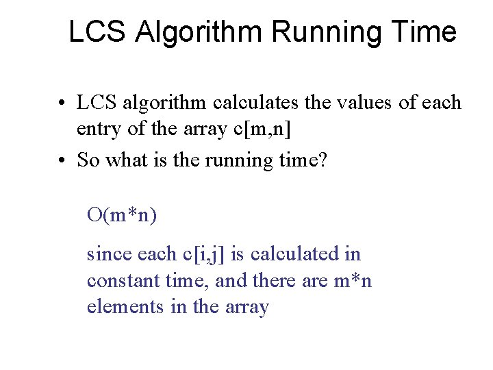
LCS Algorithm Running Time • LCS algorithm calculates the values of each entry of the array c[m, n] • So what is the running time? O(m*n) since each c[i, j] is calculated in constant time, and there are m*n elements in the array

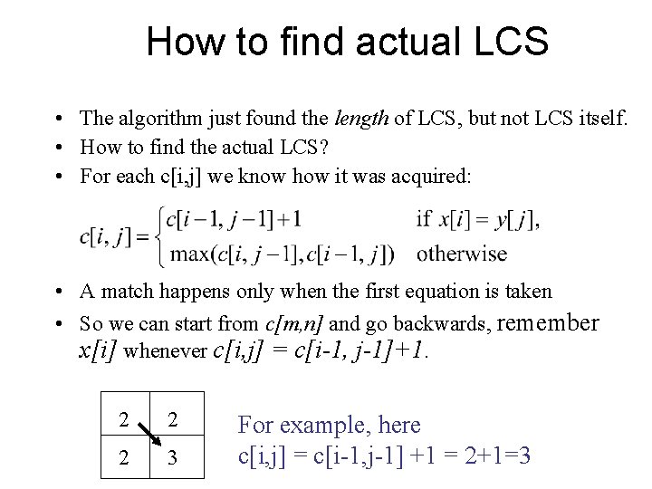
How to find actual LCS • The algorithm just found the length of LCS, but not LCS itself. • How to find the actual LCS? • For each c[i, j] we know how it was acquired: • A match happens only when the first equation is taken • So we can start from c[m, n] and go backwards, remember x[i] whenever c[i, j] = c[i-1, j-1]+1. 2 2 2 3 For example, here c[i, j] = c[i-1, j-1] +1 = 2+1=3

Finding LCS j 0 Y[j] 1 B 2 D 3 C 4 A 5 B 0 X[i] 0 0 0 1 A 0 0 1 1 2 B 0 1 1 2 3 C 0 1 1 2 2 2 4 B 0 1 1 2 2 3 i Time for trace back: O(m+n).

Finding LCS (2) j 0 Y[j] 1 B 2 D 3 C 4 A 5 B 0 X[i] 0 0 0 1 A 0 0 1 1 2 B 0 1 1 2 3 C 0 1 1 2 2 2 4 B 0 1 1 2 2 3 i LCS (reversed order): B C B LCS (straight order): B C B (this string turned out to be a palindrome)

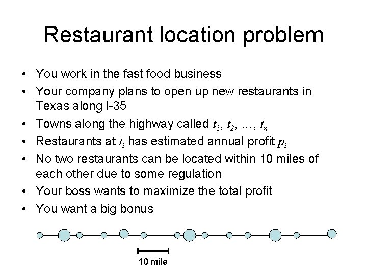
Restaurant location problem • You work in the fast food business • Your company plans to open up new restaurants in Texas along I-35 • Towns along the highway called t 1, t 2, …, tn • Restaurants at ti has estimated annual profit pi • No two restaurants can be located within 10 miles of each other due to some regulation • Your boss wants to maximize the total profit • You want a big bonus 10 mile

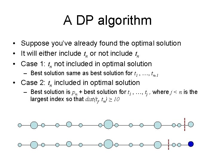
A DP algorithm • Suppose you’ve already found the optimal solution • It will either include tn or not include tn • Case 1: tn not included in optimal solution – Best solution same as best solution for t 1 , …, tn-1 • Case 2: tn included in optimal solution – Best solution is pn + best solution for t 1 , …, tj , where j < n is the largest index so that dist(tj, tn) ≥ 10

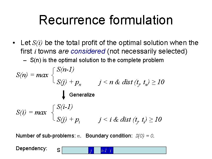
Recurrence formulation • Let S(i) be the total profit of the optimal solution when the first i towns are considered (not necessarily selected) – S(n) is the optimal solution to the complete problem S(n) = max S(n-1) S(j) + pn j < n & dist (tj, tn) ≥ 10 Generalize S(i) = max S(i-1) S(j) + pi j < i & dist (tj, ti) ≥ 10 Number of sub-problems: n. Boundary condition: S(0) = 0. Dependency: S j i-1 i

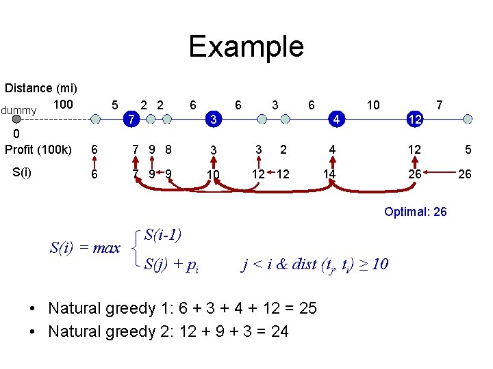
Example Distance (mi) dummy 100 0 Profit (100 k) S(i) 5 2 2 6 7 6 3 6 7 9 8 3 6 7 9 9 10 10 7 4 3 12 2 4 12 5 12 12 14 26 26 Optimal: 26 S(i) = max S(i-1) S(j) + pi j < i & dist (tj, ti) ≥ 10 • Natural greedy 1: 6 + 3 + 4 + 12 = 25 • Natural greedy 2: 12 + 9 + 3 = 24

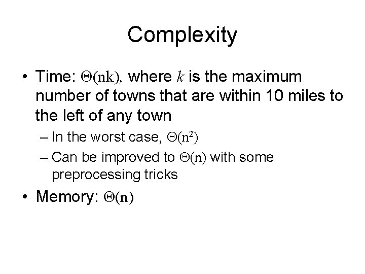
Complexity • Time: (nk), where k is the maximum number of towns that are within 10 miles to the left of any town – In the worst case, (n 2) – Can be improved to (n) with some preprocessing tricks • Memory: Θ(n)

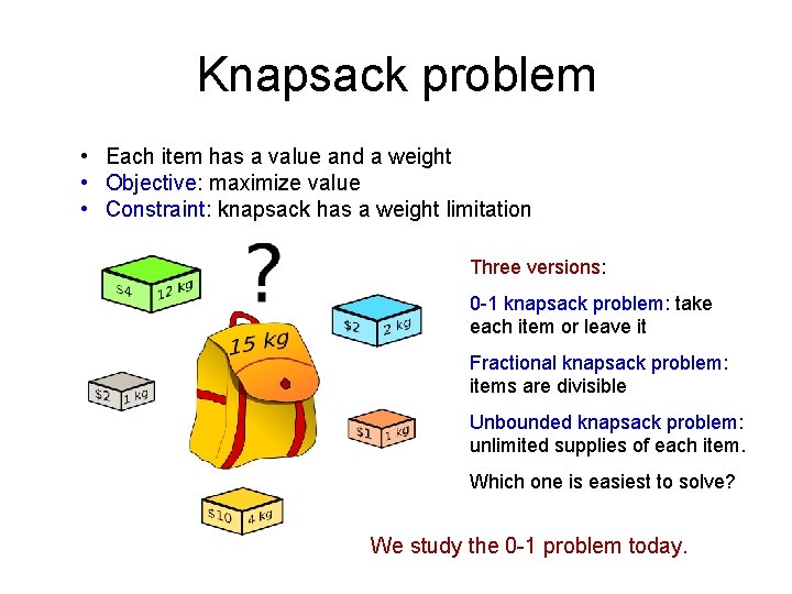
Knapsack problem • Each item has a value and a weight • Objective: maximize value • Constraint: knapsack has a weight limitation Three versions: 0 -1 knapsack problem: take each item or leave it Fractional knapsack problem: items are divisible Unbounded knapsack problem: unlimited supplies of each item. Which one is easiest to solve? We study the 0 -1 problem today.

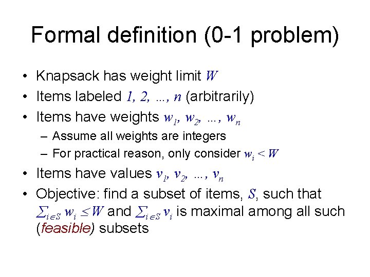
Formal definition (0 -1 problem) • Knapsack has weight limit W • Items labeled 1, 2, …, n (arbitrarily) • Items have weights w 1, w 2, …, wn – Assume all weights are integers – For practical reason, only consider wi < W • Items have values v 1, v 2, …, vn • Objective: find a subset of items, S, such that i S wi W and i S vi is maximal among all such (feasible) subsets

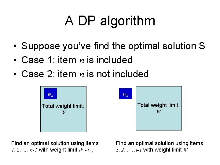
A DP algorithm • Suppose you’ve find the optimal solution S • Case 1: item n is included • Case 2: item n is not included wn Total weight limit: W Find an optimal solution using items 1, 2, …, n-1 with weight limit W - wn wn Total weight limit: W Find an optimal solution using items 1, 2, …, n-1 with weight limit W

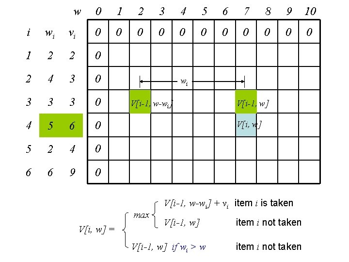
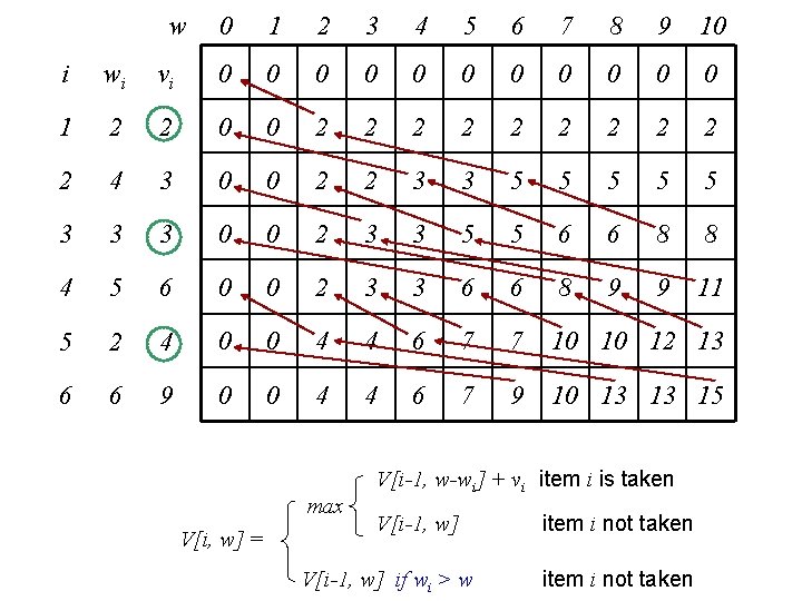
Recursive formulation • Let V[i, w] be the optimal total value when items 1, 2, …, i are considered for a knapsack with weight limit w => V[n, W] is the optimal solution V[n, W] = max V[n-1, W-wn] + vn V[n-1, W] Generalize V[i, w] = max V[i-1, w-wi] + vi item i is taken V[i-1, w] item i not taken V[i-1, w] if wi > w item i not taken Boundary condition: V[i, 0] = 0, V[0, w] = 0. Number of sub-problems = ?

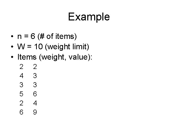
Example • n = 6 (# of items) • W = 10 (weight limit) • Items (weight, value): 2 4 3 5 2 6 2 3 3 6 4 9

w 0 1 2 3 4 5 6 7 8 9 10 0 0 i wi vi 0 1 2 2 0 2 4 3 0 3 3 3 0 4 5 6 0 5 2 4 0 6 6 9 0 wi V[i-1, w-wi] V[i, w] max V[i, w] = V[i-1, w] V[i-1, w-wi] + vi item i is taken V[i-1, w] if wi > w item i not taken

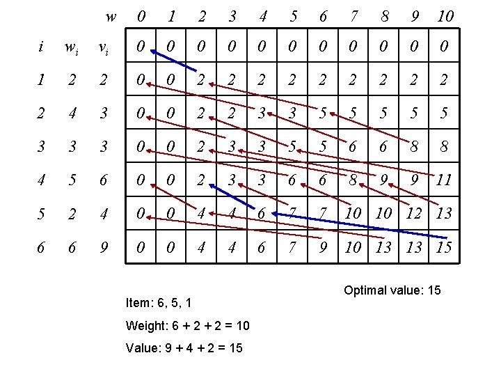
w 0 1 2 3 4 5 6 7 8 9 10 i wi vi 0 0 0 1 2 2 0 0 2 2 2 2 2 4 3 0 0 2 2 3 3 5 5 5 3 3 3 0 0 2 3 3 5 5 6 6 8 8 4 5 6 0 0 2 3 3 6 6 8 9 9 11 5 2 4 0 0 4 4 6 7 7 10 10 12 13 6 6 9 0 0 4 4 6 7 9 10 13 13 15 max V[i, w] = V[i-1, w-wi] + vi item i is taken V[i-1, w] if wi > w item i not taken

w 0 1 2 3 4 5 6 7 8 9 10 i wi vi 0 0 0 1 2 2 0 0 2 2 2 2 2 4 3 0 0 2 2 3 3 5 5 5 3 3 3 0 0 2 3 3 5 5 6 6 8 8 4 5 6 0 0 2 3 3 6 6 8 9 9 11 5 2 4 0 0 4 4 6 7 7 10 10 12 13 6 6 9 0 0 4 4 6 7 9 10 13 13 15 Item: 6, 5, 1 Weight: 6 + 2 = 10 Value: 9 + 4 + 2 = 15 Optimal value: 15

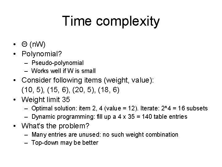
Time complexity • Θ (n. W) • Polynomial? – Pseudo-polynomial – Works well if W is small • Consider following items (weight, value): (10, 5), (15, 6), (20, 5), (18, 6) • Weight limit 35 – Optimal solution: item 2, 4 (value = 12). Iterate: 2^4 = 16 subsets – Dynamic programming: fill up a 4 x 35 = 140 table entries • What’s the problem? – Many entries are unused: no such weight combination – Top-down may be better

Use DP algorithm to solve new problems • Directly map a new problem to a known problem • Modify an algorithm for a similar task • Design your own – Think about the problem recursively – Optimal solution to a larger problem can be computed from the optimal solution of one or more subproblems – These sub-problems can be solved in certain manageable order – Works nicely for naturally ordered data such as strings, trees, some special graphs – Trickier for general graphs • The text book has some very good exercises.

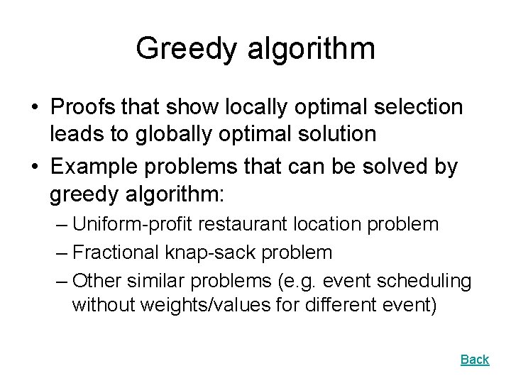
Greedy algorithm • Proofs that show locally optimal selection leads to globally optimal solution • Example problems that can be solved by greedy algorithm: – Uniform-profit restaurant location problem – Fractional knap-sack problem – Other similar problems (e. g. event scheduling without weights/values for different event) Back

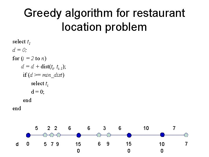
Greedy algorithm for restaurant location problem select t 1 d = 0; for (i = 2 to n) d = d + dist(ti, ti-1); if (d >= min_dist) select ti d = 0; end 5 d 0 2 2 5 7 9 6 6 15 0 3 6 6 9 10 15 0 7 10 0 7

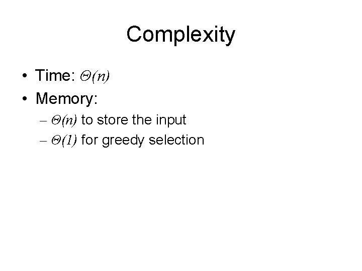
Complexity • Time: Θ(n) • Memory: – Θ(n) to store the input – Θ(1) for greedy selection

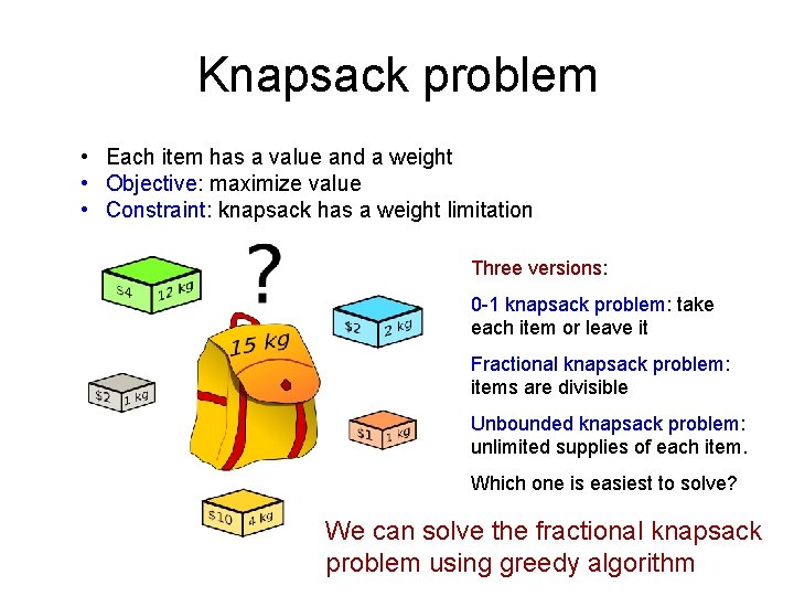
Knapsack problem • Each item has a value and a weight • Objective: maximize value • Constraint: knapsack has a weight limitation Three versions: 0 -1 knapsack problem: take each item or leave it Fractional knapsack problem: items are divisible Unbounded knapsack problem: unlimited supplies of each item. Which one is easiest to solve? We can solve the fractional knapsack problem using greedy algorithm

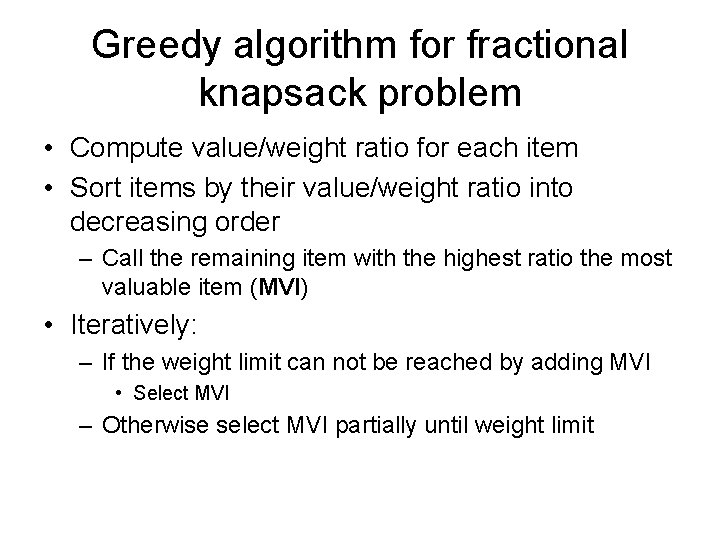
Greedy algorithm for fractional knapsack problem • Compute value/weight ratio for each item • Sort items by their value/weight ratio into decreasing order – Call the remaining item with the highest ratio the most valuable item (MVI) • Iteratively: – If the weight limit can not be reached by adding MVI • Select MVI – Otherwise select MVI partially until weight limit

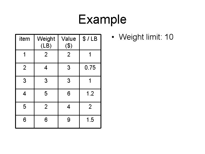
Example item Weight (LB) Value ($) $ / LB 1 2 2 1 2 4 3 0. 75 3 3 3 1 4 5 6 1. 2 5 2 4 2 6 6 9 1. 5 • Weight limit: 10

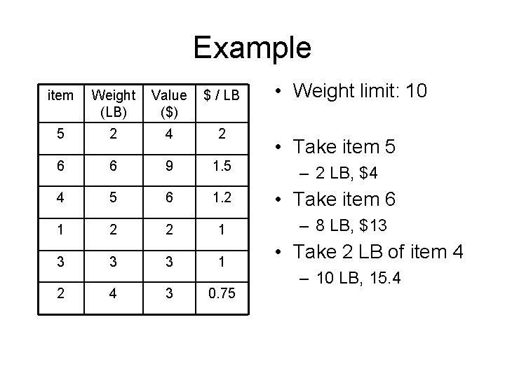
Example • Weight limit: 10 item Weight (LB) Value ($) $ / LB 5 2 4 2 6 6 9 1. 5 – 2 LB, $4 4 5 6 1. 2 • Take item 6 1 2 2 1 3 3 3 1 2 4 3 0. 75 • Take item 5 – 8 LB, $13 • Take 2 LB of item 4 – 10 LB, 15. 4

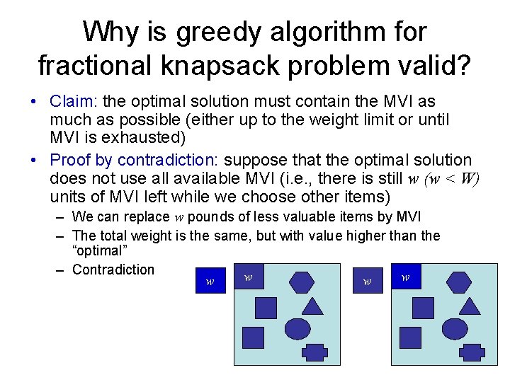
Why is greedy algorithm for fractional knapsack problem valid? • Claim: the optimal solution must contain the MVI as much as possible (either up to the weight limit or until MVI is exhausted) • Proof by contradiction: suppose that the optimal solution does not use all available MVI (i. e. , there is still w (w < W) units of MVI left while we choose other items) – We can replace w pounds of less valuable items by MVI – The total weight is the same, but with value higher than the “optimal” – Contradiction w w

Graphs • Representations – Adjacency list vs adjacency matrix – Cons and pros • MST – Kruskal’s – Prim’s Back

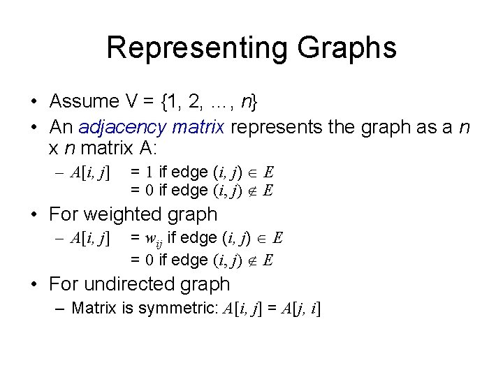
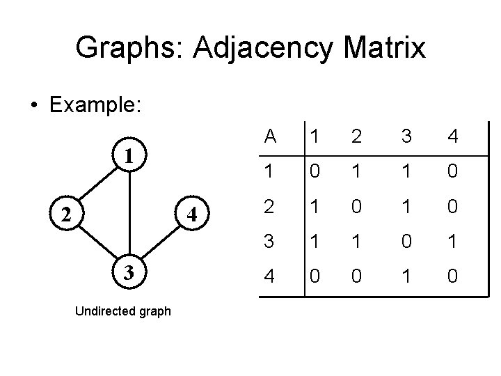
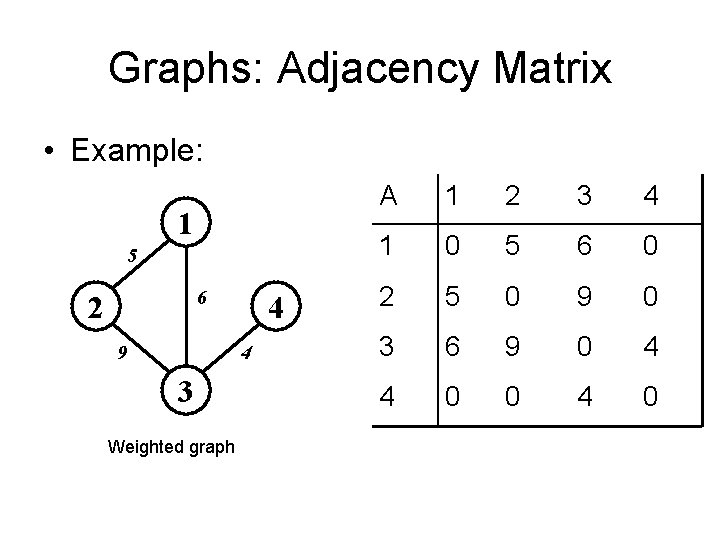
Representing Graphs • Assume V = {1, 2, …, n} • An adjacency matrix represents the graph as a n x n matrix A: – A[i, j] = 1 if edge (i, j) E = 0 if edge (i, j) E • For weighted graph – A[i, j] = wij if edge (i, j) E = 0 if edge (i, j) E • For undirected graph – Matrix is symmetric: A[i, j] = A[j, i]

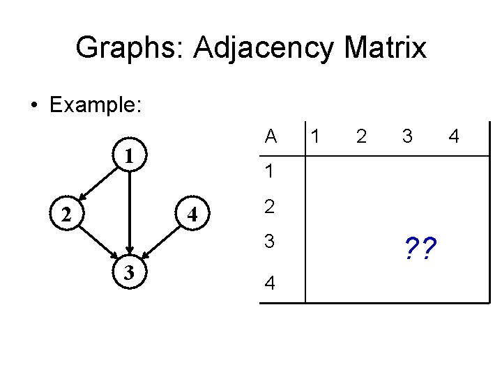
Graphs: Adjacency Matrix • Example: A 1 2 2 3 1 4 2 3 3 1 4 ? ? 4

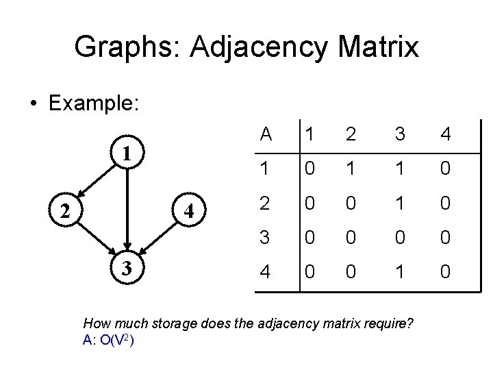
Graphs: Adjacency Matrix • Example: 1 2 4 3 A 1 2 3 4 1 0 1 1 0 2 0 0 1 0 3 0 0 4 0 0 1 0 How much storage does the adjacency matrix require? A: O(V 2)

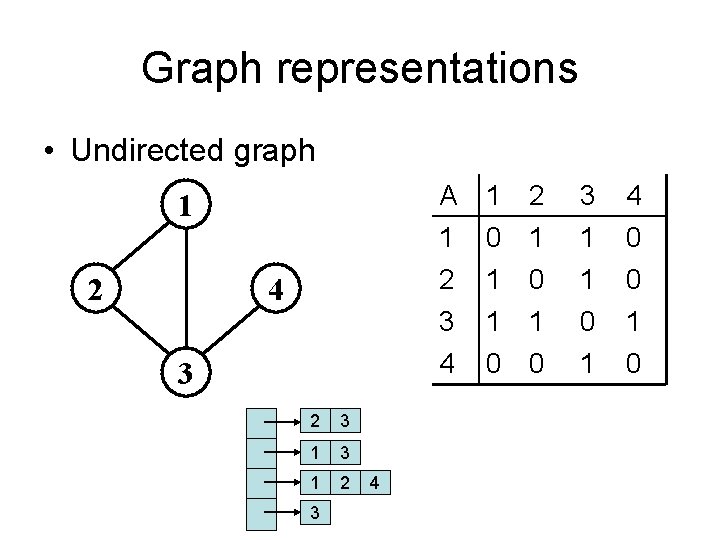
Graphs: Adjacency Matrix • Example: 1 2 4 3 Undirected graph A 1 2 3 4 1 0 1 1 0 2 1 0 3 1 1 0 1 4 0 0 1 0

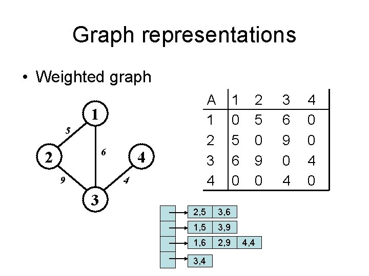
Graphs: Adjacency Matrix • Example: 1 5 6 2 9 4 4 3 Weighted graph A 1 2 3 4 1 0 5 6 0 2 5 0 9 0 3 6 9 0 4 4 0 0 4 0

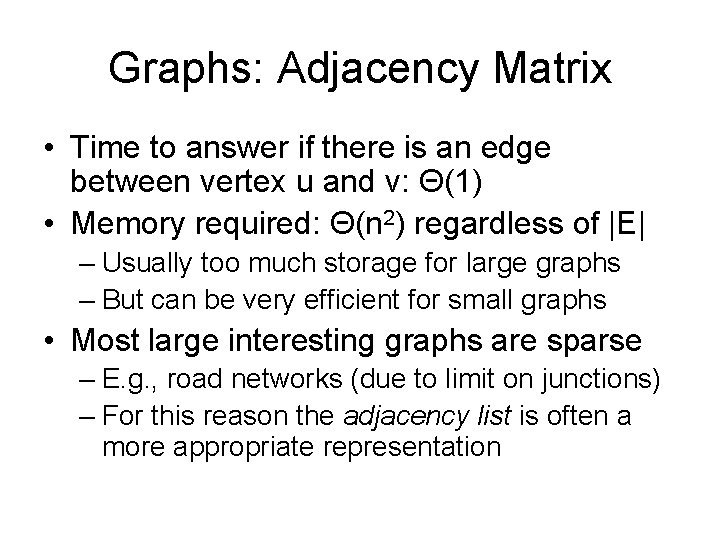
Graphs: Adjacency Matrix • Time to answer if there is an edge between vertex u and v: Θ(1) • Memory required: Θ(n 2) regardless of |E| – Usually too much storage for large graphs – But can be very efficient for small graphs • Most large interesting graphs are sparse – E. g. , road networks (due to limit on junctions) – For this reason the adjacency list is often a more appropriate representation

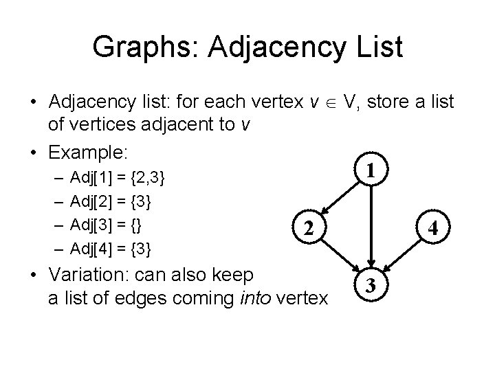
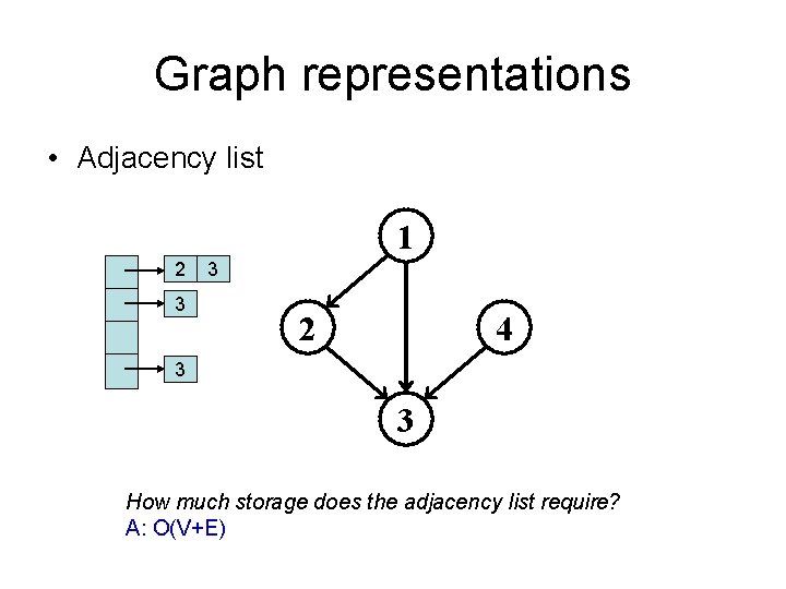
Graphs: Adjacency List • Adjacency list: for each vertex v V, store a list of vertices adjacent to v • Example: – – Adj[1] = {2, 3} Adj[2] = {3} Adj[3] = {} Adj[4] = {3} 1 2 • Variation: can also keep a list of edges coming into vertex 4 3

Graph representations • Adjacency list 1 2 3 3 2 4 3 3 How much storage does the adjacency list require? A: O(V+E)

Graph representations • Undirected graph 1 2 4 3 2 3 1 2 3 4 A 1 2 0 1 1 0 3 1 1 4 0 0 3 4 1 1 0 0 0 1 1 0

Graph representations • Weighted graph A 1 2 3 4 1 5 6 2 9 4 4 3 1 0 5 6 0 2, 5 3, 6 1, 5 3, 9 1, 6 2, 9 3, 4 2 5 0 9 0 4, 4 3 6 9 0 4 4 0 0 4 0

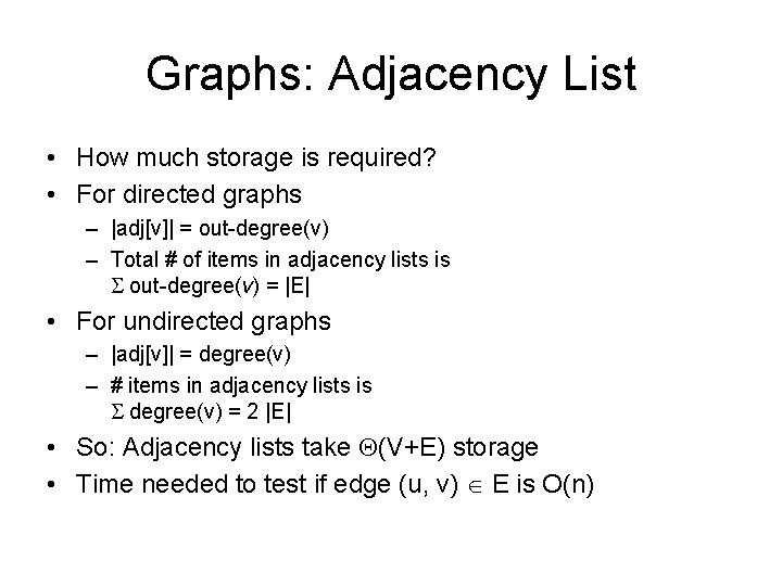
Graphs: Adjacency List • How much storage is required? • For directed graphs – |adj[v]| = out-degree(v) – Total # of items in adjacency lists is out-degree(v) = |E| • For undirected graphs – |adj[v]| = degree(v) – # items in adjacency lists is degree(v) = 2 |E| • So: Adjacency lists take (V+E) storage • Time needed to test if edge (u, v) E is O(n)

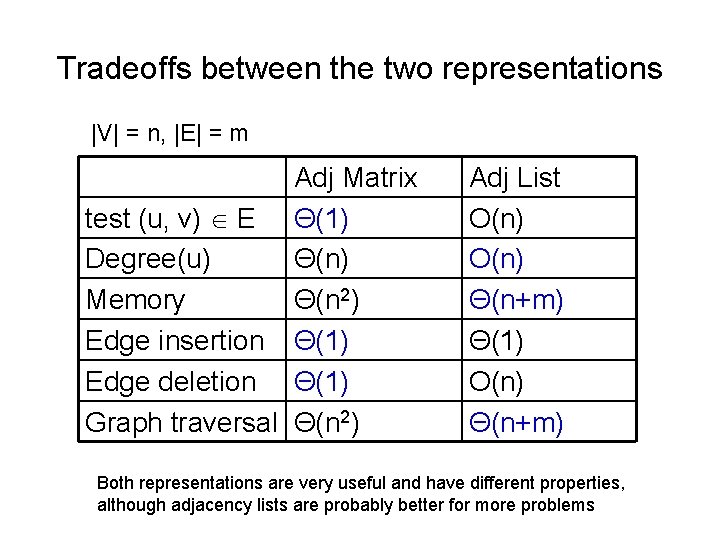
Tradeoffs between the two representations |V| = n, |E| = m Adj Matrix test (u, v) E Θ(1) Degree(u) Θ(n) Memory Θ(n 2) Edge insertion Θ(1) Edge deletion Θ(1) Graph traversal Θ(n 2) Adj List O(n) Θ(n+m) Θ(1) O(n) Θ(n+m) Both representations are very useful and have different properties, although adjacency lists are probably better for more problems

Good luck with your exam!